1.Introduction

The submerged jet flow has been a widely studied subject due to its frequent occurrence in nature and its multiple applications in engineering. Based on the Reynolds number (Re) value, two main types of submerged jet flows can be defined, namely, laminar and turbulent. Some examples of turbulent jets (Re> 3000) can be found in the breathing process in the human nasal passages (Doorly et al.¹), among others. Similarly, laminar jets (Re< 3000) can be found in the propulsion drive of some animals such as jellyfish (Vogel ²). The fundamental interest of this work is the study of the dynamics of submerged jet flows for small values of the Reynolds number (Re< 1) and the changes in the structure of the flow that take place when it leaves the tube of a given wall thickness.

To our knowledge, the first exact solutions for submerged jet flows induced by a point source of momentum within an infinite medium were proposed by Landau ³, Squire⁴ and Yatseyev ⁵.

Landau³ made the following assumptions to solve this problem analytically: the jet stream is produced by a point source of momentum, which implies that there is no mass transfer; the flow is in a steady-state; the fluid that occupies the medium in which the jet discharges and fluid injected by the jet are the same; the fluid is highly viscous; finally, the external forces that could act on the flow are not taken into account. This solution has two limiting cases, -first, when the value of Re is very low (weak flow) and -second, when the value of Re is very high (strong flow), this idealized flow was proposed as an example of an academic problem with exact solution, but it is physically unrealistic.

Regarding practical cases, some of the first experimental studies on submerged jet streams that originate from a pipe were carried out by Oberbeck , in his study, a solution of water and ink was injected vertically with ascending direction, first continuously and then intermittently, the evolution in time of the jet was sketched, the vortex ring that is generated during the very early stages of the injection process is described and changes on the structure of the jet when interacting with different obstacles, such as a sphere, a wall normal to the flow and a wall parallel to the flow, were discussed.

Similarly, Reynolds ⁷ made observations on submerged jet streams, this time, he also injected fluid vertically, but along the downward direction and described how the experimental conditions made it difficult to obtain steady flows for Reynolds numbers between 10 and 30.

Abramovich and Solan⁸ conducted experiments in the range from 80 <Re< 500, finding that the forward speed of the front is proportional to half the speed of the fluid element on the longitudinal axis of the steady jet, this velocity was measured throughout an axial distance of 40 diameters from the pipes’ outlet .

Andrade and Tsien ⁹ captured long exposure photographs of a horizontally injected jet of a fluid containing suspended particles, obtaining the velocity profile in the center-line of the jet.

Other authors have conducted experiments on submerged jet flows that originate in a hole in a wall instead of a tube. McNaughton and Sinclair ¹⁰, agree with Reynolds⁷ that the action of dyeing the fluid sensitively modifies its density, which becomes evident for small Re values (Re< 100), consequently, the fluid modifies the behavior of the jet, because the flotation and the inertial forces are of the same order of magnitude. Schneider¹¹ and Zauner¹² found two different behaviors of the jet, first, when Re> 30, the flow is perpendicular to the walls due to the viscosity, and second, when Re< 30 two toroidal eddies are formed due to the influence of the walls. Schneider¹³ presents a theoretical prediction that describes the flow with more accuracy, for these cases, compared to the Squire⁴ solution.

In more recent works on the submerged jet problem, Lemanov et al.¹⁴ studied the transition distance of the submerged jets from laminar to turbulent for 100 >Re> 600. In their experiments, they observed that the width of the jet is the same size as that of the diameter of the injector.

Hsu et al. ¹⁵ carried out experiments of a submerged jet that ensues from a pipe for Re= 39.4 and 78.8, they find that the jet flow goes in the opposite direction to the injection soon after leaving the source, this is attributed to the difference of densities between the injected flow and the surrounding environment. Lee etal. developed an analytical solution for fully developed laminar jets, by which the maximum velocity in the center of the injector can be calculated.

The aforementioned authors studied the influence on the flow structure due to the change in the value of Re number for injectors of fixed shape, nevertheless, in the present work, the effects on the flow structure due to the change in wall thickness are studied, for this purpose, the division of this work is as follows: the physical problem is stated in Sec. 2, the equations to be solved are given, as well as the conditions to which they are subject, the method used in their solution is described, likewise, the experimental configuration is described along with the procedure followed during measurements. Section 3 presents the most significant results obtained from the numerical simulations and the experimental realizations in the form of contour graphs and velocity components distribution plots, as well as the stream function value distribution; finally, in the last section, the main results obtained in this study are discussed.

2.Numerical solution and experimental study

2.1.Problem statement

In order to determine the submerged jet flow structure, the equations of continuity and Navier-Stokes (N. S.), which express the conservation of mass and momentum, respectively, were stated in cylindrical coordinates and were solved taking the following considerations: the flow is assumed to be axisymmetric; the jet emerges from a submerged circular pipe, which discharges the same fluid found in the quiescent surrounding medium; the fluid is considered to be Newtonian, incompressible, with constant viscosity and density; the flow is assumed to have reached a steady-state; the gravity force, as well as all external forces, are absent; (see the sketch in Fig. 1) leaving:

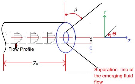
FIGURE 1 Schematic representation of the pipe outlet, spacial coordinates and geometrical dimensions. 

Continuity equation in cylindrical coordinates

1r∂(rvr)∂r+∂∂z(ρvz)=0, (1)

and the respective N.S. equation in cylindrical coordinates are coordinate r:

vr∂vr∂r+vz∂vr∂z=-1ρ∂p∂r+νu(Δvr-vrr2), (2)

coordinate z:

vr∂vz∂r+vz∂vz∂z=-1ρ∂p∂r+νΔvz, (3)

where

Δf=1r∂∂r(r∂f∂r)+∂2f∂z2. (4)

From Eqs. (1)-(3) the vorticity-stream function formulation in cylindrical coordinates is obtained

1r∂ψ∂z∂ς∂r-1r∂ψ∂r∂ς∂z-1r∂ψ∂zςr=1Re∂2ς∂z2+∂2ς∂r2+1r∂ς∂r-1r2ς (5)

where

ς=(1r2∂ψ∂r-1r∂2ψ∂r2-1r∂2ψ∂z2), (6)

And

vr=1r∂ψ∂z,vz=-1r∂ψ∂r. (7)

The equations were dimensionalized using the inner radius of the tube R and the value of the mean velocity v _mean =Q/πR ² , where the Reynolds number based on R is Re=ρv _mean R/μ. Equations (5) and (6) are the same as those used by Kanda and Shimomukai ¹⁷, in the numerical treatment of the entrance flow problem in a pipe.

2.3.Experimental set up

In order to carry out the experimental study and to analyze the submerged jet flow structure, a prismatic tank with transparent 6 mm thick acrylic walls was built with internal dimensions 11.2×11.8×60 mm (see Fig. 2), these dimensions were chosen to minimize the effects caused by the proximity of the walls to the jet flow, which can be avoided with a separation of at least 6 times the radius according to López-Villa et al., , with said separation being 17 times the inner radius for the present study. At the base of the container, an 8 mm circular hole was drilled allowing the injector pipe to pass through, to determine the injection flow rate, the left wall of the channel was marked with multiple horizontal lines with a separation of 2 mm. Four aluminum tubes were machined, all of them with an inner diameter D _in = 6.35 mm ±0.02 mm (R= 3.175 mm) and outer diameters D _out = 8 mm ±0.02 mm, 9.52 mm ±0.02 mm, 12.69 mm ±0.0.02 mm and 24.5 mm ±0.0.02 mm, and 100 mm length to achieve fully developed flow inside the pipe and produce a parabolic velocity profile (Poisseuille flow), all four pipes at the opposite end have an outer diameter of 8 mm so they can be coupled at the reservoir base.

FIGURE 2 Schematic representation of the experimental set up. 

The working fluid consisted of U.S.P. glycerin, with dissolved 20 μm polyamide, thus allowing the use of the PIV technique. The fluid was injected using a pressurized vessel, which has a capacity of 500 ml. Injection pressure for all cases was set at about 0.6 kg/cm², to obtain Re≈ 0.11 values, the pressure was measured with a Metron brand pressure gauge with a capacity of 1 kg/cm², with an accuracy of ±0.5%. The vessel was pressurized with a “maintenance free” Craftsman brand compressor, which was equipped with a moisture filter, and has a 33 Gal storage capacity. The velocity fields were video recorded with a Dantec Dynamics PIV system, and the image sets were processed using the DANTEC Dynamic Studio software. The video camera is set normal to the laser sheet, in turn, the laser sheet is placed at the middle plane of the test section, and it crosses the pipe centerline.

3.Experimental and numerical results

The main objective of the series of experiments described here is to register the shape of a submerged jet flow for a small Reynolds number (Re= 0.11) and to describe how said shape changes with increasing the wall thickness of the injector. The above is achieved by using four nozzles with the same internal diameter but different wall thicknesses e (corresponding to e=R/4, R/2, R and 3R).

Three important changes in the shape of the jet, which can be observed with the naked eye, are presented in Fig. 3. First, the change in the exit angle β of the flow at the injector mouth, this angle decreases with the thickness of the injector wall (see Fig. 4); second, as the flow moves away from the injector along the line of symmetry, the jet acquires a constant radius (upper part of the jet), which increases as the thickness of the tube wall grows; and finally, the size of the recirculation zone (the region of fluid dragged by the jet) is also modified, the occurrence of these regions of the flow is caused by the presence of the walls of the test section, it is observed that the size and the position of the core of these re-circulation zones change with the thickness of the tube wall.

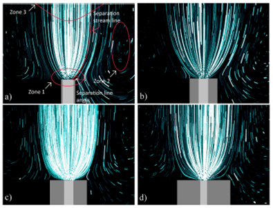
FIGURE 3 Long exposure pictures of a submerged jet at Re = 0:11, t = 600 s, for: a)D _in = 6:3 mm, e = R=4, b) D _in = 6:3 mm, e = R=2, c) D _in = 6:3 mm, e = R, and d) D _in = 6:3 mm, e = 3R. 

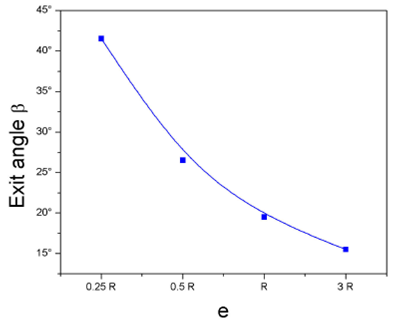
FIGURE 4 Plot of the decrease of the exit angle β when changing the thickness of the nozzle of the injector to Re = 0:11. 

In Fig. 5, the distribution of the axial velocity component along the line of symmetry (maximum velocity) obtained from the experimental measurements is compared to the distribution produced by the numerical method developed for this study.

FIGURE 5 Plot of the maximum speed drop vs. distance (r) at Re = 0:11. 

In the numerical simulation, the change in the distribution of the axial velocity component that results from modifying the thickness of the tube is almost imperceptible, so the only distribution presented is the one corresponding to the thickest tube (e= 3R).

The axial velocity component distribution in the radial direction, at the positions R/2, R, 2R, 3R, 4R, and 5R, starting at the mouth of the tube, along the line of symmetry, were obtained, for a value of Re= 0.11, as shown in Figs. 5-12. In these plots, it is observed that by increasing the thickness of the wall of the tube, the width of the jet increases, causing the profile of the axial component of speed to contract in the axial direction and to elongate in the radial direction.

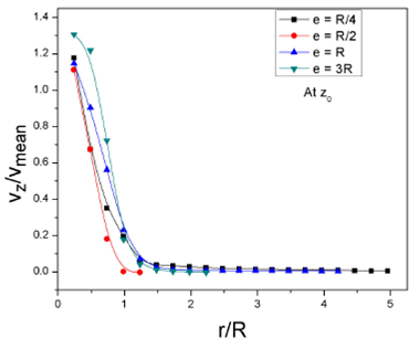
FIGURE 6 Plot of the axial velocity component profile along the radial direction at the injector outlet (z ₀) at Re = 0:11. 

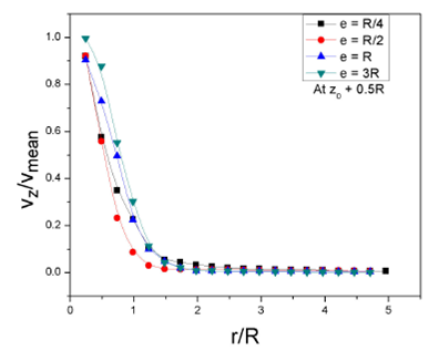
FIGURE 7 Plot of the axial velocity component profile at z ₀+0:5R distance from the nozzle outlet at Re = 0:11. 

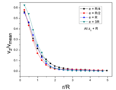
FIGURE 8 Plot of the axial velocity component profile at z ₀ + R distance from the injector outlet at Re = 0:11. 

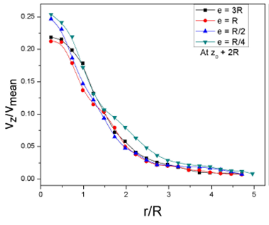
FIGURE 9 Plot of the axial velocity component profile at z ₀ +2R distance from the nozzle outlet at Re = 0:11. 

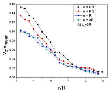
FIGURE 10 Plot of the axial velocity component profile at z0+3R distance from the nozzle outlet at Re = 0:11. 

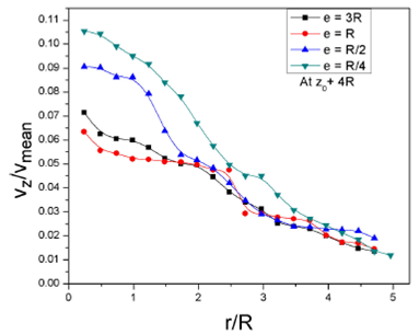
FIGURE 11 Plot of the axial velocity component profile at z0+4R distance from the injector outlet at Re = 0:11. 

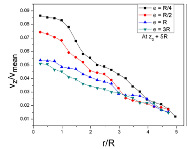
FIGURE 12 Plot of the axial velocity component profile at z0+5R distance from the injector outlet at Re = 0:11. 

Level curves of the dimensionless values of the velocity magnitude, the radial and axial components of the velocity, are placed side by side in Figs. 13 -15. Even though results were obtained for the four wall thicknesses, only the results for the case where e= 3R are presented. Similarly, in Figs. 16, the distribution of the axial velocity component along the radial direction at various positions along the symmetry line, as obtained experimentally, are compared with the numerically calculated values.

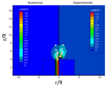
FIGURE 13 Comparison of the velocity magnitude distribution for Re = 0:11; e = 3R, as obtained numerically and experimentally. 

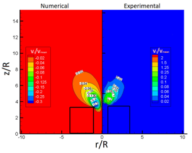
FIGURE 14 Comparison of the radial velocity component distribution for Re = 0:11; e = 3R, as obtained numerically and experimentally. 

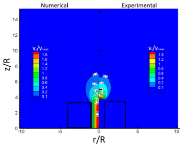
FIGURE 15 Comparison of the axial velocity component distribution for Re = 0:11; e = 3R, as obtained numerically and experimentally. 

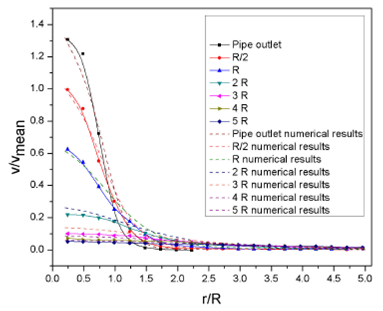
FIGURE 16 Comparison of the profiles of the axial velocity component along the radial direction at various distances from the nozzle outlet, for Re = 0:11; e = 3R, as obtained numerically and experimentally. 

To distinguish the main jet flow from the surrounding medium, it is considered that the jet, at all times, has the same volumetric flow rate as that occurring inside the tube.

The value of the stream function in the simulation is known since the numerical code that resolves the velocity is based on the vorticity-stream function formulation, which calculates the value of the stream function and subsequently derives the value of the velocity components.

To determine the value of the stream-function from the experimentally obtained values of the velocity components, a numerical code was developed, with a procedure similar to that described by Roache .

The value of the stream function corresponding to the separation streamline for the numerical simulation and the integration of the experimental results, is 0.5 and 0.48, respectively (see Fig. 17).

FIGURE 17 Comparison of the stream-function (PSI) distribution for Re = 0:11; e = 3R, as obtained numerically and experimentally. 

4.Discussion and conclusions

The structure of submerged jet flows originating from a circular tube and the actual effects that modifying the wall thickness of the tube has on such flows, for a given Reynolds number (Re= 0.11), were the studied experimentally and numerically. After comparing results, the following conclusions were reached:

It is considered that the change in the structure of the flow is translated into the change in the region of influence of the jet. It is expected that, at low Reynolds numbers, the fluid flow will be reversible, thus allowing to take samples from specific fluid regions.