


 text new page (beta)
 English (pdf)
 Article in xml format
 Article references
 Send this article by e-mail
 Cited by SciELO
  Similars in
SciELO
Similars in
SciELO 
 Permalink
1. Introduction
Creep compliance is a material property that relates a continuous deformation of a specimen when subjected to a constant stress. Basically, a creep test consists on applying a constant load to a test specimen for certain period of time, and the strains that it suffers are measured and registered [1]. The creep compliance of elastomers has been determined by using different experimental test methods; for example: the ASTM-D2990 and ISO 899-1:2003 standard methods, non-standardized tensile tests [2] and dynamic-mechanical analysis (DMA) [3], in which the strains are measured by using displacement sensors located at mobile grips. In general, the testers employed in these test methods are very complex and they have different limitations for creep strain measurement. Thus, more reliable and accurate techniques to measure creep strain in elastomers are required. Full field optical techniques could be an alternative for these measurements since they yield more information of the strains over the object surface.
Digital speckle shearing interferometry also known as shearography is a full field interferometry technique used to determine the surface displacements derivatives [4]. For many engineering disciplines is important to measure the strain and related parameters. Shearography has been implemented to measure surface strain showing some significant advantages over other interferometry techniques, such as the elimination of the reference beam of holography and the necessity of a special vibration insolation [5]. These advantages have converted shearography into a practical strain measurement tool. Consequently, it has already received wide acceptance for nondestructive testing [6,7]. Besides, some applications of shearography reported are: the evaluation of delamination in tires, nondestructive test in aircraft structures, evaluating debond in composite structures, evaluation of residual stress, 3D shapes measurement, vibrations analysis and strain measurement [8-10]. This technique has proven to be a relatively low-cost [11]. Besides that it is easy to adapt in many applications, it can be potentially used to determine some mechanical properties of materials [12,13].
In this paper, authors have explored the application of shearography for the evaluation of creep in elastomers. Three elastomers were tested in this work: neoprene/chloroprene (CR), ethylene-propylene diene monomer (EPDM) and Fluoroelastomer (FKM). In order to demonstrate the adaptability of shearography for the measurement of creep strains, an in-plane shearography setup was implemented in a simple short-term tensile creep test (3 hours). Finally, the results obtained from shearography are compared with that obtained with commercial digital image correlation (DIC) equipment.
2. Theory
2.1. Creep
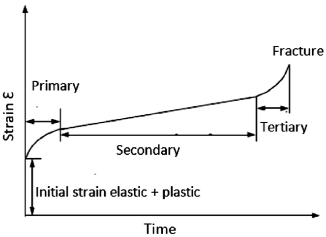
Creep is a slow continuous deformation of a material under constant stress [1]. A characteristic creep curve consists of three different stages as shown in Fig. 1. The first stage in which creep occurs at a decreasing rate is called primary creep. The second creep stage, called the secondary stage, proceeds at a nearly constant rate; and the third or tertiary stage occurs at an increasing rate finishing in fracture. The total strain ε at any instant of time t in a creep test is represented as the sum of the instantaneous elastic strain ε e and the creep strain ε c :
Commonly, the creep behavior is reported as creep compliance, which is the ratio between the creep strain and the applied stress. It may be defined by:
where ε(t) is the creep strain and σ 0 is the stress.
In some design calculation for polymers, it is common to use the creep modules E(t) instead of elastic modulus E of the material. For a prolonged constant load, the creep modulus varies with time, showing a decay in this property due to a rearrangement of the polymer chains [14,15]. The creep modulus, E c , is defined by:
2.2. Electronic speckle pattern shearing interferometry (shearography)
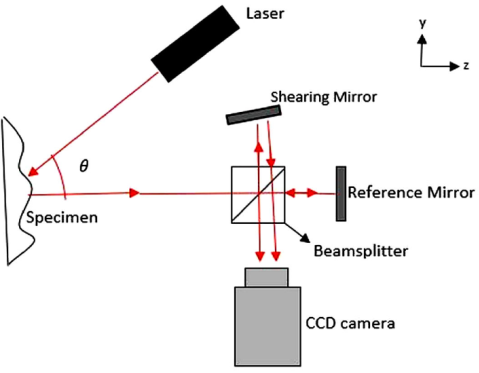
Since its invention, shearography has been used in many applications [16,17]. Some of these applications are vibration analysis, curvature measurement, and full-field measurement of displacement derivatives [18-20]. These applications have defined shearography as a well stablished non-destructive technique [21]. A typical shearography arrangement to measure the out-of-plane displacement derivatives is shown in Fig. 2. This is the most common setup for non-destructive testing. An expanded laser beam illuminates the specimen surface. The scattered light forms a speckle pattern which is captured by a charge-coupled device (CCD) camera through a modified Michelson interferometer [5]. One of the mirrors of the Michelson interferometer is slightly tilted in order to form two sheared images of the object surface.
The interference of the two sheared images will result in a shearing speckle pattern. Although, intensity and phase are spatial dependent variables, the notation of this dependency is omitted in order to make the equations more compact. The intensity of this speckle pattern may be expressed as:
where I is the intensity distribution of the speckle pattern, I 0 is the average intensity, μ is the modulation of the speckle pattern, and φ is a random phase angle. When the object is deformed, an optical path change occurs due to the surface displacement of the object. This optical path change induces a relative phase change between two interfering points. Thus, the intensity distribution of the speckle pattern is slightly altered and is described by the following equation:
where I ’ is the intensity distribution after deformation, and φ ’ denotes the phase change due to the deformation.
In order to conduct a quantitative analysis, the phase distribution has to be determined. To measure the phase distribution, a phase-shifting technique must be implemented [6,7,22]. Some phase-measuring algorithms have been developed, such as the three, four, and five-step phase shifting algorithms. However, the most common phase shifting algorithm is the four steps [23]. In this algorithm, four images with a corresponding phase shift of π / 2 are captured. These phase changes are introduced by translating one of the mirrors in the modified Michelson interferometer using a piezo-electric crystal (PZT). Thus, the four resulting intensities are expressed as:
Solving the four last equations, the so called wrapped phase is obtained:
This process is repeated for the deformed state of the specimen. So, at the deformed state the phase φ ’ is obtained. Subtracting the phase φ ’ from φ, the relative phase difference Δ is obtained. This relative phase difference is related to the total deformation of the object surface. However, the resulting phase from Eq. (10) consists of discontinuities due to the tangent function. So, a phase unwrapping algorithm has to be applied to obtain a continuous phase distribution [24].
For an illumination beam, the relationship between the phase change and the derivatives of displacements is given by the next equation [25]:
where λ is the laser wavelength, θ is the angle of illumination, δ y is the amount of shear in the y direction, ∂w=∂y and ∂v=∂y are components of derivatives of displacement. From Eq. (11), it can be seen that there are both, in-plane and out-of-plane, components of derivatives displacements. For non-destructive testing, the out-of-plane, component is usually isolated. This is achieved by setting at almost zero the angle of illumination. However, for strain analysis, the in-plane component of the displacement derivative most be isolated. For this, an in-plane shearography setup is necessary. With the in-plane optical setup, only the ∂v=∂y component will remain [26-28]. A typical in-plane shearography setup is shown in Fig. 3. In this arrangement, the object surface is sequentially illuminated by two symmetrical incident beams. The phase shifting procedure is implemented for each beam separately. As a result, two phase relative differences are obtained:
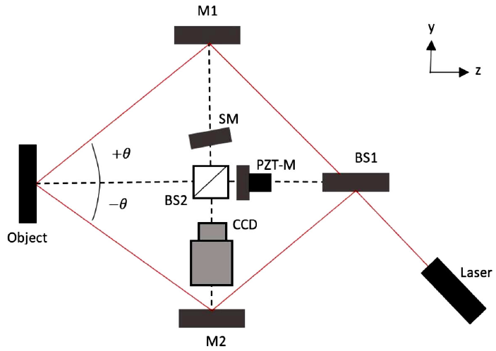
Figure 3 In-plane shearography arrangement. M1 and M2: mirrors, SM: shearing mirror, PZT-M: piezo crystal mirror, BS1 and BS2: beam splitters, +θ and -θ: incident angles.
Subtracting Eq. (12) from Eq. (13), finally the in-plane strain component is obtained:
From Eq. (15) it can be seen that it is necessary to obtain first the phase distribution corresponding to each beam separately at the state of reference and at the deformed state.
3. Experimental details
In this paper, the fluoroelastomer (FKM), neoprene (CR), ethylene-propylene-dine monomer (EPDM) elastomers were evaluated. These polymers are regularly used to fabricate static and dynamic seals for machinery [29]. The samples were extracted from commercial flat and thin black sheets. They were cut in dumbbell shape according to the standard method for tension tests of rubber materials as established in the ASTM D 412 [30]. The gauge of the specimens forms a rectangle with a length of 30 mm and a width of 3.5 mm. The specimens were fully painted with white paint to give more visibility to the laser speckles. Also, they were characterized according to tensile breaking stress and tear strength. In Table I these mechanical properties are reported. These test for characterization were conducted according to the ASTM-D412 procedure for tensile breaking stress by using a tensile tester with a load cell of 900 N, and the ASTM-D624 method was carried out to obtain the tear strength by using the same tensile tester.
Table I Mechanical properties of FKM, CR and EPDM.
| Elastomer | Thickness [mm] | Tensile breaking stress [MPa] | Tear strength [KN/m] |
|---|---|---|---|
| Fluoroelastomer, FKM | 1 ± 0.01 | 8.8 ± 0.3 | 2.53 ± 0.23 |
| Neoprene/Chloroprene, CR | 2.9 ± 0.01 | 10.7 ± 0.8 | 6.34 ± 0.15 |
| Ethylene-Propylene-Diene Monomer, EPDN | 3 ± 0.01 | 5.9 ± 0.3 | 9.47 ± 0.3 |
In this work, short term creep tests with a duration of three hours were conducted. A dead load of 1.5 N was applied to each elastomer. The stress generated by this load was calculated according to the cross section of the specimens, being 0.44 MPa for FKM, 0.15 MPa for CR and 0.135 MPa for EPDM. The specimen was clamped to a structure and the dead load was manually and gently applied to its bottom by using a dead weight fixed with a binder clip.
The shearography arrangement employed to measure the creep strain in polymers is shown in Fig. 4. The light source is a Helium Neon laser with λ = 633 nm. The laser beam is expanded with a microscope objective (MO). Then, mirror 1 (M1) reflects the light to the beam splitter 1 (BS1), which splits the light into two separate beams. Beam 1 (B1) and beam 2 (B2) are reflected by mirror 2 (M2) and mirror 3 (M3) respectively, and they reach the specimen surface with an angle of 18.5 degrees. In front of the sample, the shearography system is installed. In the Michelson interferometer, the mirror 5 (M5) is slightly tilted to obtain a shearing distance of 5 mm in the y direction. This shearing distance represents the 16.6% of the length of the specimen’s gauge. Apparently, this distance is relatively large for an approximation to the derivative; however, if this distance is reduced, the quality of the phase distribution is affected. Moreover, with this shearing distance, results obtained showed agreement with another measurement method, as will be seen further. In mirror 4 (M4) a PZT crystal is incorporated to carry out the four steps phase shifting. It was found that a 3.17 V is required to produce a phase shift of π / 2. For the image acquisition, the Pixellink PL-B953F CCD monochrome camera was used. The camera is a 0.8 mega pixel (1024 × 768). The camera lens used was the Navitar zoom 7000 with a focal length of 18-108 mm and F-number of 2.5. The camera was positioned at a distance of 400 mm and is focused on the gauge of the specimen through the beam splitter 2 (BS2) with a focal length of 108 mm, a F# of 8 and a magnification of 0.15. The image acquisition and the phase shifting were controlled by a program written in LabVIEW software and the image processing was performed using the MATLAB software. For the wrapped phase, a sine/cosine average filter was used; and the unwrapped phase was calculated by using the MATLAB unwrapped algorithm.
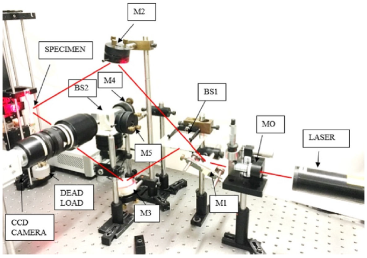
Figure 4 Arrangement of the shearography system: M1 through M5: mirrors; MO: microscopy objective; BS1 and BS2: beam splitters.
Although shearography is relatively insensitive against the small rigid-body motion (few microns), the large rigid-body motion could lead to speckle decorrelation, which could introduce considerable errors to the measurements [11]. So, the measurements were initiated after 30 seconds when the specimen was stabilized. For CR and EPDM the sampling was performed every minute during 30 minutes. After 30 minutes, measurements were performed every 3 minutes until complete 3 hours. Due to FKM is subjected under a higher stress and therefore it suffers more strain compared with CR and EPDM, the sampling was effectuated every 30 seconds during the first 30 minutes. After that, the measurements were done every minute for 30 minutes until to complete 1 hour. For the last 2 hours, the sampling was performed every 3 minutes until complete 3 hours. In the image processing, it was observed that a decorrelation occurred every 5 minutes during the first 30 minutes. So, the reference image was changed every 5 measurements, and the strain obtained was progressively summed. After 30 minutes, as the deformation occurred relatively slower, decorrelation occurred every 12 minutes, being the strain also progressively summed. Two creep tests were carried out for the three materials to see repeatability in the data.
4. Results and discussions
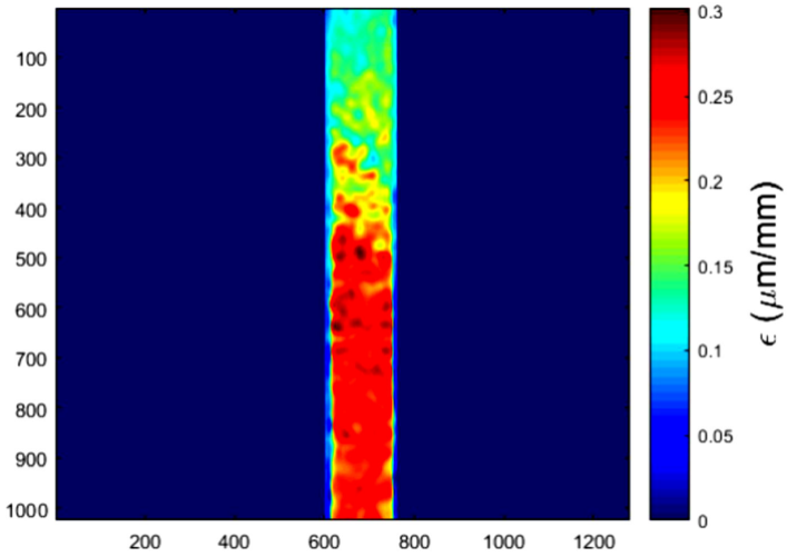
During the image processing, it was important to measure the strain only from the gauge length of the specimens. Thus, a rectangular mask was created over the specimen as shown in Fig. 5. The average value of the strains on this area was computed, and by using the Eq. (2), the creep compliance was calculated. The results of creep compliance for the two tests are shown in Fig. 6.
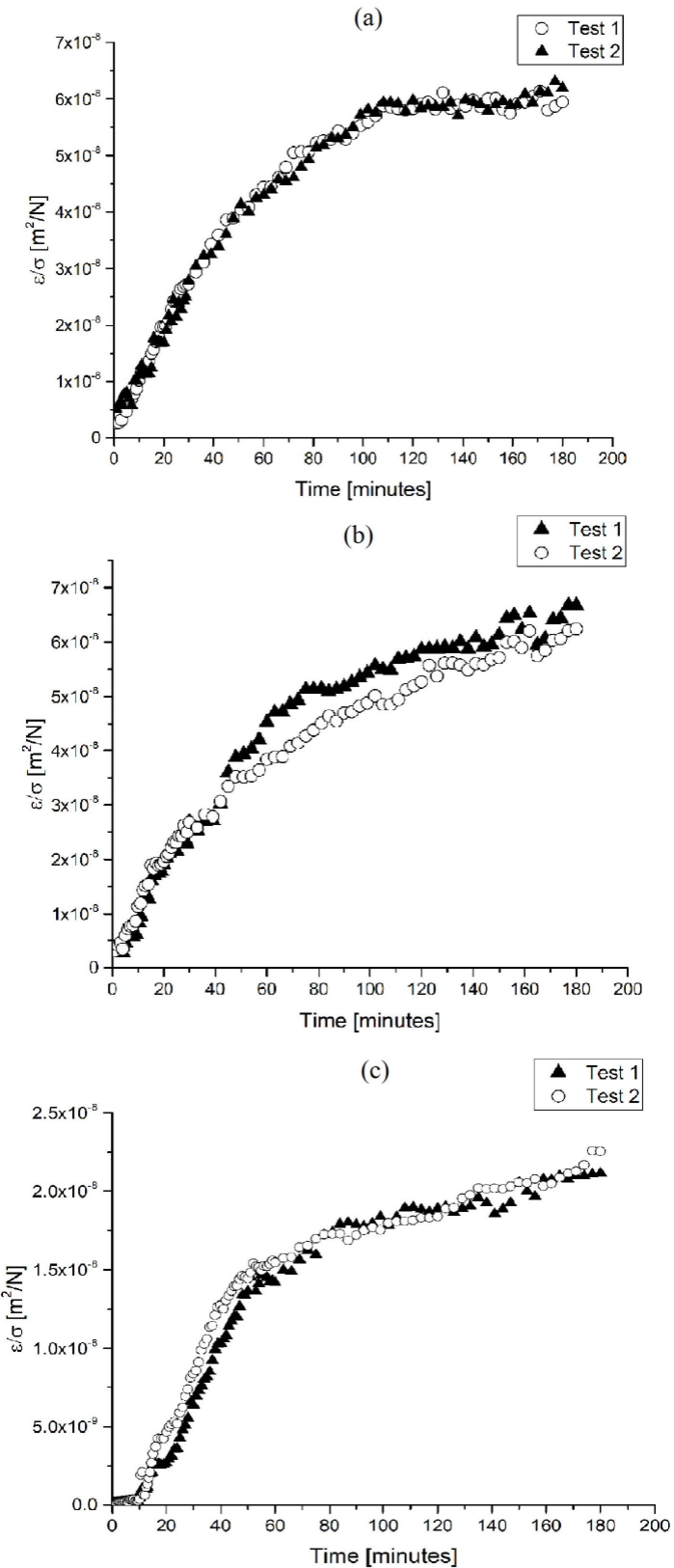
Since this shearography setup cannot measure large instantaneous strains, the initial strain was omitted in the calculation of creep compliance in Fig. 6. However, the initial strain in a creep test could be predicted by using the mean elastic modulus of the material, or even can be neglected [1]. Also, in Fig. 6 it can be observed that the two tests performed for each material presented a similar tendency. Moreover, in the plots of creep compliance, it can be also seen that the three materials presented an expected linear viscoelastic behavior [14]. In order to validate the results, the same experiments were conducted by using a DIC equipment for strain measurement. As well as the case of shearography, in order to evaluate the strain distribution with DIC, a rectangle mask was created over the gauge of the specimen. In Fig. 7 a characteristic strain distribution obtained with DIC is presented. A comparison of creep strain of the three elastomers obtained with each method can be observed in Fig. 8.
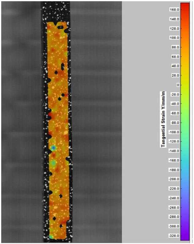
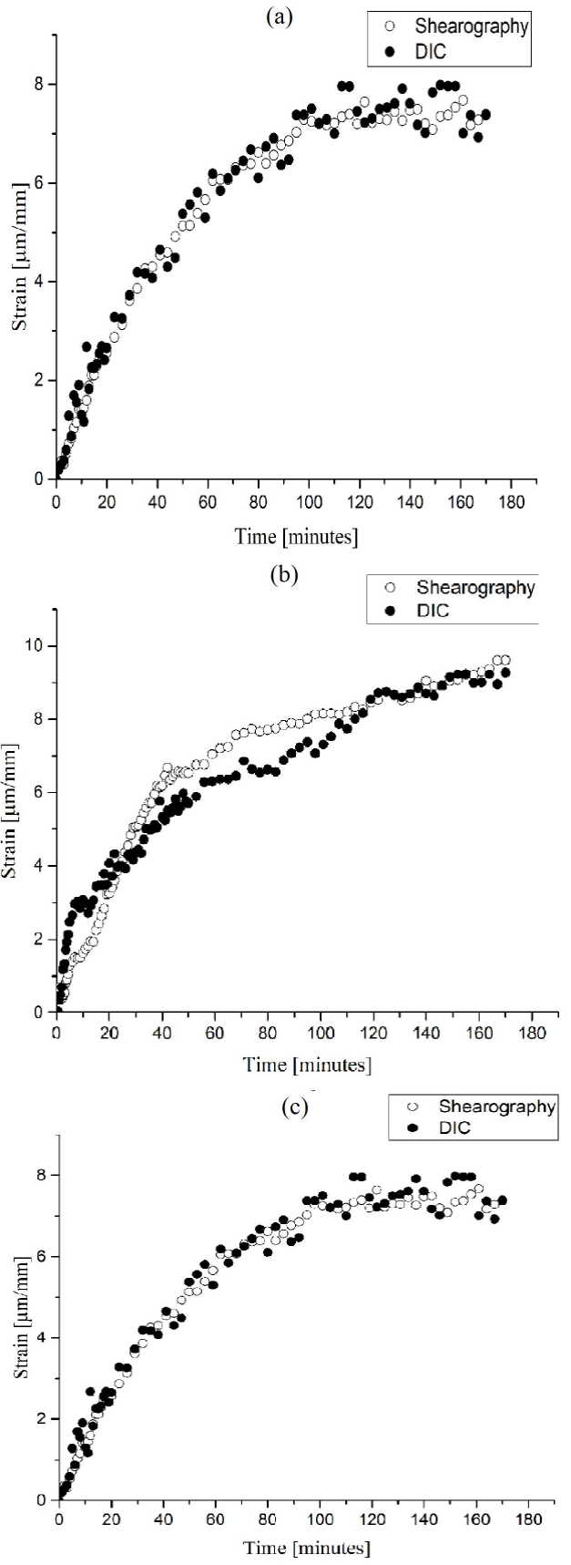
Figure 8 Comparison of creep strain obtained with shearography and DIC for: (a) CR, (b) EPDM and (c) FKM.
From the graphs shown in Fig. 8 it can be seen that the results obtained with both optical methods are very similar, and they show agreement with the expected characteristic creep curve for polymers. Also, from the curves in Fig. 8 the primary stage of creep can be clearly observed. Besides, it is also visible the initiation of the secondary stage of creep (in which the strain rate is nearly constant) at the minutes 100 for FKM and CR and 150 for EPDM.
As mentioned above, this experimental shearography setup is not able to measure the instantaneous strains, because elastomers suffer large strains and rigid-body motion when the load is applied. This is the principal limitation of this technique for the study of creep. However, it can be over-come by calculating the initial strain using the mean elastic modulus of the material. Moreover, if long-term experiments are conducted, it is also possible to obtain the secondary stage and even the tertiary stage of creep for polymers.
In Table II the percentage differences between shearography and DIC measurements at different times for the three materials are reported. It can be seen that the results are similar.
5. Conclusions
Shearography was applied to measure strains in elastomers. An in-plane shearography setup was implemented to measure creep strain in FKM, CR and EPDM. Results obtained with shearography were compared with that obtained with a commercial digital image correlation equipment. The creep results obtained by using both techniques were very similar and they match with the characteristic idealized creep curve imposed for elastomeric materials. Although this shearography set up showed some drawbacks, such as the inability to measure large and instantaneous strains and its high sensibility to rigid-body motion, it was demonstrated that it could be used as an alternative tool to measure strain in creep tests where the initial strain can be neglected. Moreover, this optical technique can be extended to the study of creep in a wide range of viscoelastic material.

