1. Introduction

A small single-axis magnetic probe (also known as B-dot) has been designed and constructed to measure the pulsed magnetic field in a Circular Demountable Toroidal Field Coil (CDTFC) [¹]. Similar phenomena like electromagnetic thrusters [²], lightning in transmission lines [³], magnetic field compression by puff-gas Z pinches [⁴], nano-second high voltage generation, high electrical current measurements in pulsed power systems [⁹], radio-frequency plasma measurements [¹⁰], and many other pulsed transient experiments make use of B-dot probes. Measurement of these pulsed transient phenomena can be a challenging task when the probe must be sensitive to all three components of the magnetic field, have enough sensitivity to detect low magnetic fields of some Gauss, and in some cases have a good response in frequency of some GHz. In our case, a pulsed magnetic field measurement in a single axis of a CDTFC in frequencies up to 20 kHz is required.

The B-dot probes for electromagnetic thrusters in aerospace applications must be able to have a frequency response of up to 100 kHz [²]. For pulsed magnetic measurements such as lightning in transmission lines [³] it is necessary a frequency response of up to 2.5 MHz. Magnetic field compression studies by puff-gas Z pinches [⁴] need magnetic field measurements that last 300 ns in time. To measure both high currents and voltages in pulsed power systems [⁹] a calibrated B-dot probe up to 4 GHz in frequency is required. B-dot probe calibration in exploding plasmas [⁶] reaches 50 MHz. Messer et al., [⁷], as well as Reilly and Miley [¹⁰], were able to calibrate B-dot coils reaching frequencies as high as 100 MHz using network analyzers.

A network analyzer is a very common device to calibrate a B-dot probe to the frequency response [⁶, ⁷,¹⁰]. Other methods such as pulsed-power RLC discharge [⁸] at high voltage at select frequencies provide relevant magnetic field magnitudes over the range of relevant frequencies to calibrate.

Helmholtz coil and short pieces of wire arrangements are the common magnetic field source generators. A Helmholtz coil applied as a magnetic field source for calibration is a reliable device due to its relative facility in construction and because the magnetic field produced in its axial axis is relatively constant. If the analytical expression of the magnetic field [⁵] produced in the axial axis center of the Helmholtz coil is expanded in series, the calculated error is 1.5 × 10 ^-4 %. A Helmholtz coil employed as a magnetic field source for calibration can operate up to 500 kHz [⁶]. When the frequency range demanded is above 500 kHz, a short piece of wire is implemented [³,⁶]. In most cases, B-dot calibration is carried out at relevant frequencies of interest [⁶,⁷,⁹] without so much attention focused on magnetic field magnitudes [⁸], assuming that B-dot sensitivity remains constant in a very wide range of magnetic field magnitude.

Recently, new methods of B-dot coils construction embedded in printed circuit boards (PCBs) are gaining popularity in applications for identifying the radiation sources in PCBs and the prediction of electromagnetic compatibility of electronic circuits according to Sivaraman [¹¹]. These new B-dot probes are tailored to operate in a frequency range from 1 MHz to 1 GHz. The aforementioned author states that, as the length of the transmission line connected to the probe increases, the probe output contains noise due to induced voltages on the transmission line. In order to reject induced voltages due to the transmission line, some methods in compensated probes as center tapped transformers, hybrid combiners or inherent pick-up rejections have been implemented [¹²] in tiny B-dot probes made with magnet wire, whereas problems in B-dot based on PCBs picking up induced voltages are solved by varying the length of the B-dot transmission line in a determined frequency range.

Other techniques to map electromagnetic fields exist besides the B-dot probe method, such as the Modulated Scattering Technique (MST), Electro-Optic Sampling (EOS), and Electron Beam Probing (EBP). These last techniques are characterized as complex ones for applications in electromagnetic field measurements [¹¹]. Therefore, a low complexity technique can be advantageous, such as the B-dot probe adopted in this work. Furthermore, EBP and EOS methods have a slow speed in relation to B-dot probe and MST, whereas these two latter ones have a medium speed. In terms of accuracy, the MST response is low, B-dot has a medium response, and the EBP is high. Thus, the most attractive advantages of B-dot probes are the relative facility of construction, the familiar method to calibrate them by using a Helmholtz coil in a relative long frequency range, and finally a relative high accuracy.

In this work a B-dot coil calibration intended to measure pulsed magnetic fields in a CDTFC [¹] is presented. The calibration is made by using a LC _var resonant circuit. The LC _var circuit is fed with a half bridge converter to stable frequencies with an Integrated Circuit (IC) IR2153 used as a driver. This IC provides a square signal with a 50% duty cycle to frequencies up to 100 kHz. The resonant relation ω = 1/√LC is used to produce sinusoidal waves at different frequencies by varying C _var , whereas the Helmholtz coil inductance L remains constant. The use of sinusoidal oscillators can replace complex equipment like network analyzers in calibration procedures at low frequencies. The oscillator type presented here is able to deliver relative high currents that produce relative high magnetic fields which are necessary to calibrate tiny B-dot probes presented in this work.

This article is structured as follows: In Sec. 2 we describe the selected parameters of a B-dot probe in order to design a suitable model able to have a range frequency response from 6.16 kHz to 36.63 kHz. In Sec. 3 we describe the characteristics of the Helmholtz coil and the resonant circuit. In Sec. 4 we explain the theory and the calibration method, whereas in Sec. 5 the sensitivity results are reported. Finally, our conclusions, as well as further discussion, are presented in Sec. 6.

2. B-dot design and construction

The herein proposed B-dot coil, presented schematically in Fig. 1, complies with the relation 0 ≤ d=2r _H ≤ 0.2, where d = 2.95 mm is the B-dot diameter and 2r _H = 62 mm is the Helmholtz coil diameter. If d=2r _H < 0.2, the magnetic field produced by the Helmholtz coil is relatively constant [²]. The quotient for B-dot/Helmholtz coil is d=2r _H = 0.0476 in our case.

Figure 1 Cross-sectional schematic view of the B-dot probe. 

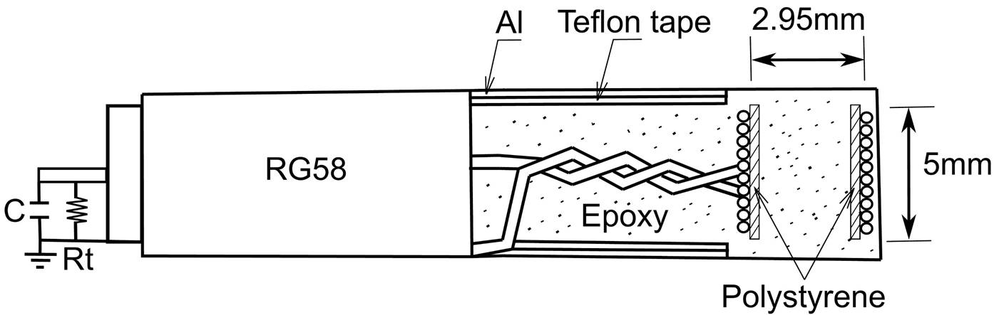
A polystyrene (μ _r ~ 1) core with d = 2.95 mm and 5 mm height is used to wrap 15 turns of magnet wire AWG34 to form the B-dot coil. The B-dot coil terminals are twisted 10 mm and connected to a coaxial cable RG58 as shown in Fig. 1. The B-dot coil is encapsulated with an epoxic resin in the cylindrical shape afforded by the coaxial cable. Teflon tape and an aluminum sheet are used to wrap the total twisted magnet wire longitude to avoid external noise. A C = 79 pF capacitance is estimated according to the probe oscilloscope and the RG58 coaxial cable longitude. A terminal resistor R _t = 670.4 Ω is connected at the end of the coaxial cable points. The terminal resistor R _t value was selected to avoid excessive voltage signal attenuation during data acquisition. This terminal resistor is also useful to damp overvoltages in the B-dot coil that could stress its turns and, in a worst-case-scenario, melt the wire.

The B-dot coil has an internal resistance R _i = 0.23 Ω and an inductance of L _i = 0.7 μH. An impedance meter U1733C was used to determine these B-dot parameters.

3. Helmholtz coil and resonant circuit

The B-dot coil calibration is carried out with a Helmholtz coil as already mentioned. The later, used as a magnetic field source, is adequate for frequencies in the range f < 500 kHz [⁶]. For higher frequencies the Helmholtz coil inductive impedance reduces the electrical current magnitude because of the skin effect, which produces magnetic field values difficult to detect for the B-dot coil during the calibration with the available laboratory equipment.

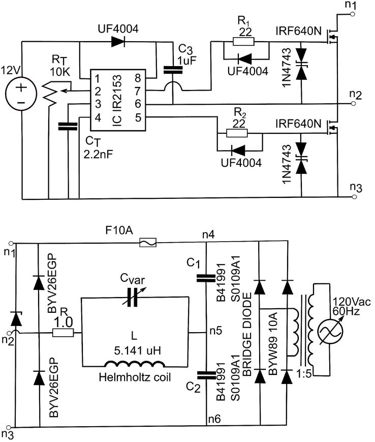
The Helmholtz coil used in this calibration has N = 3 turns, an internal resistance of R _H = 0.07 Ω, an inductance L = 5.14 μH, and a radius r _H = 0.03 m. A capacitor bank C _var connects in parallel with the Helmholtz coil L through nodes n ₂ and n ₅ in order to form a resonant circuit LC _var by varying C _var as shown in Fig. 2. An oscillator circuit of a half-bridge kind coupled to an Integrated Circuit (IC) IR2153 feeds the LC _var terminals, thus generating sinusoidal voltage waves at various frequencies. LC _var circuit is connected through the terminals n ₁, n ₂ and n ₃ to the coupled half-bridge oscillator and IC driver IR2153 whose main features are its internal dead time to avoid cross conduction in the MOSFETS and its capacity to produce train pulses at different frequencies by modifying R _t value. The fast switching MOSFETS combined with the driver IR2153 allow to drive relative high currents (up to 20 A) in the LC _var tank circuit. This LC _var operates with ac polypropylene film capacitors able to manage the currents in the Helmholtz coil at the reported frequencies. The LC _var coupled with IR2153 is able to work up to 36.63 kHz without presenting distortions in the sinusoidal waves. The driver IR2153 is capable to produce square signals up to 100 kHz but LC _var tank is unable to resonate at those relative high frequencies due to capacitance variations in the polypropylene capacitors. The half-bridge circuit stage is some tens cm apart from the LC _var tank circuit in order to minimize electromagnetic radiation from the MOSFETS switching operation.

Figure 2 Half-bridge circuit oscillator coupled with IC IR2153 feeds LC _var . 

4. Theory and calibration method

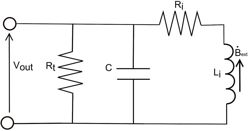
A lumped parameter circuit model for the B-dot coil is shown in Fig. 3. Applying both Kirchhoff Voltage Law (KVL) and Kirchhoff Current Law (KCL) to this lumped circuit, an induced input voltage anḂ _ext is obtained, which can be written in terms of the output voltage V _out as

where a is the B-dot probe area, n is the number of turns, R _i is the B-dot probe internal resistance, R _t is a terminal resistor, C is the internal capacitance, M is the mutual inductance, L _i is the internal inductance and Ḃ _ext is the rate of change of the magnetic field produced by the Helmholtz coil arrangement. Taking the Fourier transform of Eq. (1) we obtain

where ρ = R _i =R _t and τ = (L _i + M)=R _t . When ω is large, the real and imaginary parts of the Eq. (2) fall off like 1/ω ² and 1/ω, respectively. At high frequencies a capacitor behaves as a short circuit, so this capacitance can be used to provide a frequency limit. For ρ ≪ 1 and ωCR _t ≪ 1, Eq. (2) can be rewritten as

whose frequency range is 0 < ω ≪ 1/R _t C. In the low frequency range (ωτ ≪ 1) Eq. (3) can be expressed in the time domain as

Therefore, Eq. (4) expresses the output voltage in the B-dot coil terminals as the product of na and the time derivative of the magnetic field B _ext .

Figure 3 Lumped circuit parameter B-dot coil model. 

The magnetic field generated by the Helmholtz coil [⁵] can be written as

where I is the electrical current that passes through the Helmholtz coil, N = 3 is the number of turns, and r _H is the Helmholtz coil radius previously defined in Sec. II. The electrical current I depends directly on the voltage value V _H , measured at the Helmholtz coil terminals shown in Fig. 2. For narrow bandwidth applications [²] where the probe sensitivity is approximately constant over the frequency range of interest, such as those considered in this work, the sensitivity β (ω) can be expressed as the ratio of the integrated output voltage V _out and the magnetic field B _ext

Thus, the sensitivity is a function of the B-dot probe output voltage V _out and the output Helmholtz coil voltage V _H . The sensitivity can also be obtained by applying the fast-Fourier transform technique (FFT) [²] to the ratio V _out and Ḃ _ext .

Thus, the sensitivity β(ω) is defined by

If there is a significant variation of the sensitivity function (in either amplitude or phase) over the expected frequency range in the application, Eq. (6) can be employed to construct a general, calibrated β(ω) over the measurement range of interest [²].

The voltages V _H and V _out are obtained simultaneously from a typical arrangement of the Helmholtz/B-dot coils as shown in Fig. 4. The B-dot probe axial axis is aligned with the axial axis of the Helmholtz coil. The Helmholtz coil output voltage V _H is a sinusoidal wave and is in phase with the output voltage V _out of the B-dot probe when the LC _var circuit is in a resonant state. The magnetic field B _ext produced by the Helmholtz coil depends on its output voltage V _H .

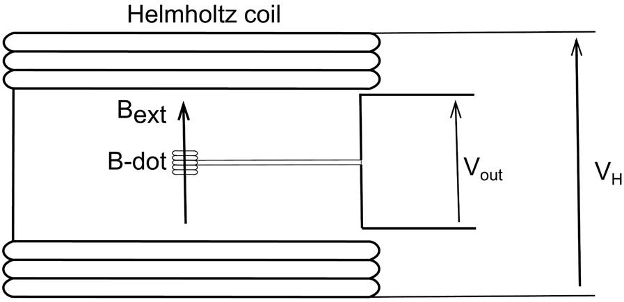
Figure 4 Typical arrangement of the Helmholtz/B-dot coils to obtain the voltages V _H and V _out 10.19 kHz. 

Alignment of the axial axis of the B-dot coil and the Helmholtz coil is carried out by rotating the B-dot coil around a perpendicular axis with respect to the axial axis of the Helmholtz coil. If V _H is a sinusoid (resonant state), the output voltage V _out of the B-dot coil is also a sinusoid in phase with V _H and the two coils are aligned when the maximum output voltage in the B-dot coil is obtained in the oscilloscope. Thus, a correlation exists between the maximum output voltage V _out in the B-dot coil and the maximum magnetic flux that passes through it.

5. Results

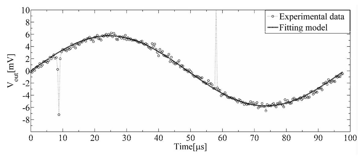
The output B-dot coil voltage wave V _out is obtained from the typical arrangement of the Helmholtz/B-dot depicted in Fig. 4. In Fig. 5 are shown both the experimental data and the output of the fitting model. The later is calculated using the least squares method, being the fitting function V _out = 0.0058sin(62900t). It can be readily seen that noise is present in the experimental data near 10μs and 60μs; this noise in the signal appears when the B-dot coil has no aluminum blindage.

Figure 5 B-dot coil output voltage V _out at a frequency of 10.19 kHz. 

Simultaneously, the output Helmholtz coil voltage V _H , depicted in Fig. 6, is also a sinusoidal wave at the same frequency as the V _out presented in the previous figure. The fitting model in this case is V _H = 3.13sin(62900t), as is also shown in Fig. 6. Using Eqs. (6) and (7), as well as the sine waves shown in Figs. 5 and 6, we obtain a sensitivity value of β ₂(ω) = 1.05 × 10 ^-4 . All sensitivities corresponding to the other frequency values are calculated in the same way.

Figure 6 Helmholtz coil output voltage V _H at the same frequency as in Fig. 5. 

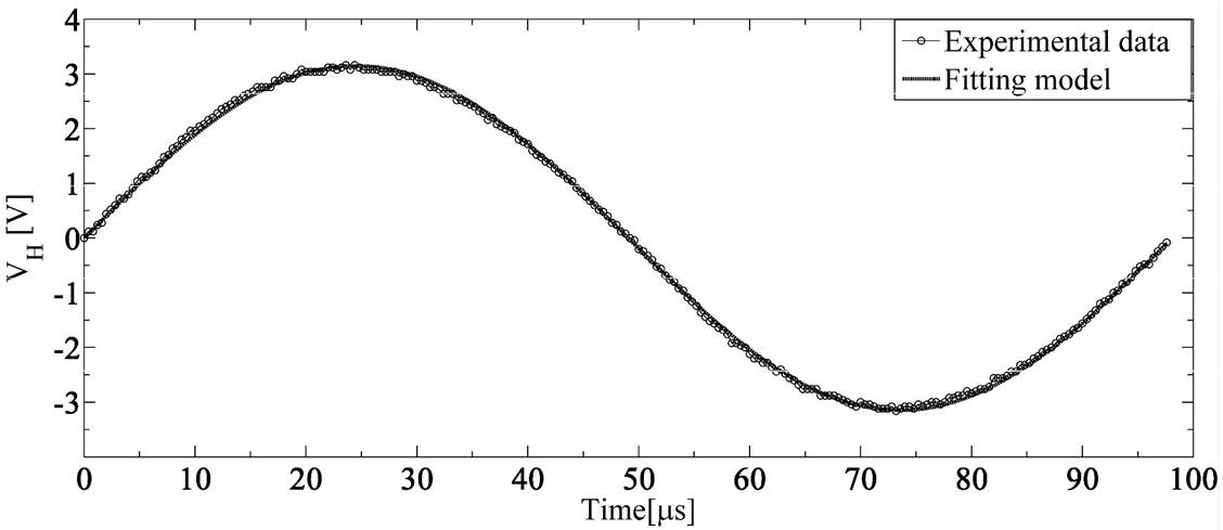
Table I shows the sensitivities for some discrete frequencies by applying Eqs. (6) and (7). F FT is also employed to calculate sensitivities. F FT sensitivity values correlate well with those determined with Eq. (6).

6. Discussion and conclusions

The sensitivity values reported in Table I experience almost no change in the frequency range from 6.16 kHz to 36.63 kHz. The “an” B-dot coil product is 1.02 × 10 ^-4 turns×m²; this value is in the same order as those in Table I. The sensitivity values reported in this table are obtained when both V _H and V _out are in phase. The B-dot coil works in the reported frequency range in a derivative mode as shown by the resultant Eq. (4) presenting a calculated offset of 9:8 × 10 ^-4 V and a power consumption in the LC _var tank circuit of ~28 W.

It is known that a decrease in the size of the B-dot coil causes a decrease in its sensitivity [¹¹]. In order to counteract sensitivity problems in relative tiny B-dot coil designs such as those studied in the present work, an increase in the magnetic field during the calibration is achieved by increasing the electric current passing through the Helmholtz coil. Higher currents are possible by implementing this half-bridge oscillator circuit. Thus, stronger magnetic fields are easily detected by the B-dot probe in terms of the B-dot voltage output as shown in Fig. 5. The half-bridge oscillator avoids the use of special equipment such as network analyzers, at least in the frequency range reported in this work. Higher currents with higher frequencies (100 kHz) are challenging to reach and are out of the scope of our work.

For frequencies above 36.63 kHz, a notorious phase displacement was found between B-dot coil and Helmholtz coil output voltages. Probable causes of this phase displacement are electromagnetic interference and external electrical couplings. The linear response of the B-dot coil is calculated for every frequency as the ratio between the peak input voltage and the peak output voltage. Taking the Helmholtz coil peak voltage as the input and the B-dot coil peak voltage as the output, a ratio value of 0.0018 is obtained from Figs. 5 and 6. This value is in good agreement with the other reported frequencies, except for the first one reported in Table I, whose ratio is 0.0023, thus experiencing a small deviation of 0:0005. Nonlinear effects are present when the ratio between the aforementioned voltages begin to change; this means that both the Helmholtz coil voltage and B-dot coil voltage sine waves are not in phase and are distorted. The reason of this phase displacement and distortion is due to the Helmholtz coil overheating that causes oscillation instabilities in the tank circuit.

The calibrated B-dot coil by this method can be used to measure pulsed magnetic field in the frequency range reported on the Table I. For the case of diagnose of high-frequency pulse trains in digital systems or high frequency oscillations, B-dot probes with similar sizes as those reported in this work have been calibrated and tested successfully in RF plasmas where sinusoidal oscillations [¹²] reach frequencies up to 13.56 MHz. B-dot probe response under transients caused by switching operations have also been tested in a switchable LRC circuit [⁶] that emulates an Alfvèn wave (100 G and 50 kHz). In order to test our B-dot coil response at higher frequencies and under switching events, especial equipment such as network analyzers have to be employed for calibration.

This B-dot coil design is planned to be used in the future to measure pulsed magnetic fields in a demountable toroidal field coil prototype. Mapping the magnetic field in different points will be useful to evaluate the performance of the demountable toroidal coil sections. Future efforts in this single axis B-dot coil design will be put into extend its bandwidth and improve the calibration constant β(ω).