


 nueva página del texto (beta)
 Inglés (pdf)
 Artículo en XML
 Referencias del artículo
 Enviar artículo por email
 Citado por SciELO
  Similares en
SciELO
Similares en
SciELO 
 Permalink
1. Introduction
Fractional calculus is a generalization for derivatives and integrals of integer order. This mathematical representation has successfully been utilized to describe several problems in engineering practices [1-7]. In the literature, there are many definitions of fractional derivative, the most popular definitions are of Riemann-Liouville, Liouville-Caputo, Caputo-Fabrizio, Atangana-Baleanu, Riesz, Hilfer, among others [8-10]. Recently, several numerical methods have been proposed to obtain approximate solutions of fractional ordinary differential equations and fractional partial differential equations, such as the fractional sub-equation method [11,12], the Adomian decomposition method [13-15], the Homotopy perturbation method [16,17], the variational iteration method [18-21], homotopy perturbation transform method [22,23], and so on.
Khalil in [24], introduced a new definition of derivative called the “conformable derivative”, this derivative satisfied some conventional properties, for instance, the chain rule, product rule, quotient rule, mean value theorem and composition rule and so on. This derivative may not be seen as fractional derivative but has fractional compound. This new operator has attracted considerable attention in recent years [25-34].
Recently a generalized definition proposed by Atangana in [35] appeared in literature on conformable derivatives. This conformable derivative is called the β-derivative. This novel derivative depends on the interval on which the function is being differentiated. Some interesting works involving these conformable derivatives have been reported in [36-39].
The β-derivative is defined as [35]
Some properties for the proposed Atangana’s-derivative are:
I) Assuming that, a and b are real numbers, g ≠ 0 and f are two functions α-differentiable and α ∈ (0; 1] then, the following relation can be satisfied
II) For any given constant “’ c” it is satisfied that
III)
IV)
Considering ∊ = (x+(1/Γ(α))) α−1 h, and h→0, when ∊ →0, therefore we have
with
where l is a constant.
V)
The proofs of the above relations are given by Atangana in [35]
The conformable-time nonlinear perturbed RadhakrishnanKundu-Lakshmanan (RKL) equation that serves as an alternate model for the propagation of light pulses and the dynamics of light pulses. This model has been studied since many years by a variety of methods that led to the retrieval of bright and dark optical solitons. This equations have the following form
where a, b, ρ, λ, θ, γ are coefficients, and φ(x,t) represent the complex-valued functions of independent variables x and t that represents the spatial and temporal variables respectively. The first, second and third terms represents the evolution term, the group velocity dispersion and the nonlinear term. Table I presents the parameters involved in Eq. (9).
Table I Description of parameters in Eq. (9).
In recent years many researchers have extensively studied different methods to obtain optical soliton solutions for RKL equation. Consequently, several methods are reported in the literature mainly in case of standard derivatives as:
For instance, in [40-41] the 1-soliton solutions of this equation are obtained by using solitary wave ansatz. New auxiliary equation method and extended simple equation method are two integration schemes used in [42] to carry out the integration of this model. The work of [43] is devoted to extract some optical soliton solutions to the model with Kerr and power laws of nonlinearity by means of extended trial function scheme. Bright, dark and singular soliton solutions of the model with two types of Kerr and power law nonlinearities are derived in [44]. Their study is based on trial equation method and modified simple equation method. Moreover, some chirp-free bright optical soliton solutions of the model is presented by traveling wave hypothesis in [45]. Lie group analysis is also used in [46] to retrieve optical soliton solutions of the perturbed Radhakrishnan-Kundu-Lakshmanan equation. In [47], the authors investigated the conformable time-fractional perturbed RKL equation by utilizing the extended sinh-Gordon equation expansion method.
Recently, generalized exponential rational function method (GERFM) has been successfully used to retrieve different types of optical soliton solutions to several nonlinear models. This powerful integration scheme also provide a guideline to classify the types of these solutions [48,49].
In this work, we will make use of the GERFM for solving the perturbed RKL Eq. (9) in the sense of the β-conformable derivative as given by Atangana [35]. To the best of our knowledge RKL equation with this kind of fractional derivative has not been solved by this scheme in the recent literature.
2. Overview of GERFM
1. Let us take into account the nonlinear partial differential equation (NPDE) in the following form
Using the transformations ψ = Ψ (τ) and τ = (σ/α) (x + (1/Γ(α)) α - (l= α))(t + (1=Γ(α))) α t, is possible reduce the NPDE to the following ordinary differential equation:
where the values of σ and l will be found later, and prime notation means the derivative of Ψ with respect to τ.
2. Consider Eq. (12) has solution of the form
where,
The values of constants p i ; q i (1 ≤ i ≤ 4), A 0 , A k and B k (1 ≤ k ≤ M) are constants to be determined, such that solution (13) satisfies Eq. (12). By considering the homogenous balance principle the value of M can be determined.
3. Substituting Eq. (13) into Eq. (12) and collecting all terms, the left-hand side of Eq. (12) is converted an algebraic equation P (Z 1 ; Z 2 ; Z 3 ; Z 4) = 0 in terms of Z i = e qiτ for i = 1, ... , 4. Setting each coefficient of P to zero, a system of nonlinear equations in terms of p i , q i (1 ≤ i ≤ 4), and σ, l, A 0 , A k and B k (1 ≤ k ≤ M) is generated.
4. Solving the above algebraic equations using any symbolic computation software, the values of p i , q i (1 ≤ i ≤ 4), A 0 ; A k , and B k (1 ≤ k ≤ M) are determined. Replacing these values in Eq. (13) one can obtain the soliton solutions of Eq. (11).
3. Analytical solution of the nonlinear Radhakrishnan-Kundu-Lakshmanan equation with β-derivative
To solve Eq. (9), we apply the following travelling wave transformation
where φ(x, t) represents the phase component, ω is the frequency of solitons, κ represents the wave number and v represents the velocity.
Substituting Eq. (15) into Eq. (9) we have the real component as
and the imaginary part as
3.1. Application of GERFM
Balancing the terms of u 3 and u ’’ in Eqs. (16) and (17) gives M= 1. Hence, from Eq. (13), we obtain:
where Φ(τ) is giving by Eq. (14).
Substituting Eq. (18) into Eqs. (17) and (16), following to method described in Section 2, we achieved the following non-trivial solutions of Eq. (9) as:
Set 1: We obtain p = [2 − i,−2 − i,−1,1] and q = [i,−i,i,−i], which gives
We also get
and
Substituting above values into Eqs. (18) and (19), we have
Therefore an exact solution of Eq. (9) is obtained as
where γ (3 λ + 2 θ) > 0 for valid soliton. Figures 1a)-1d) and 2a)-2b) show the soliton surface and the 2D graph for Eq. (25), respectively.
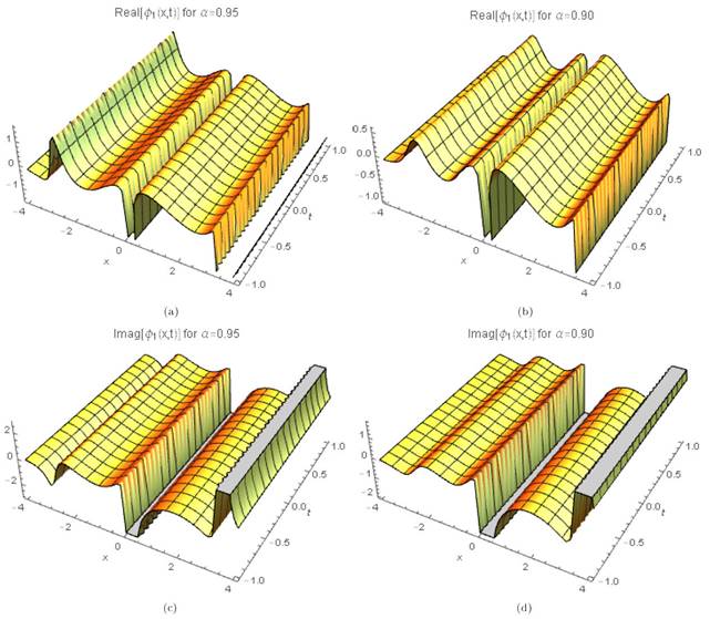
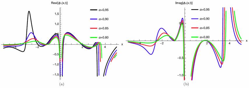
Figure 2 2D Plot soliton solution for Eq. (25) for different particular cases of ρ, arbitrarily chosen.
[Set 2:] We obtain p = [i, -i, 1, 1] and q = [i, -i, i, -i], which gives
We also get
and
Substituting above values into Eqs. (18) and (26), we have
Therefore an exact solution of Eq. (9) is obtained as
where γ(3 ‚ + 2 θ) > 0 for valid soliton. Figures 3a)-3d) and 4a)-4b) show the soliton surface and the 2D graph for Eq. (32) respectively.
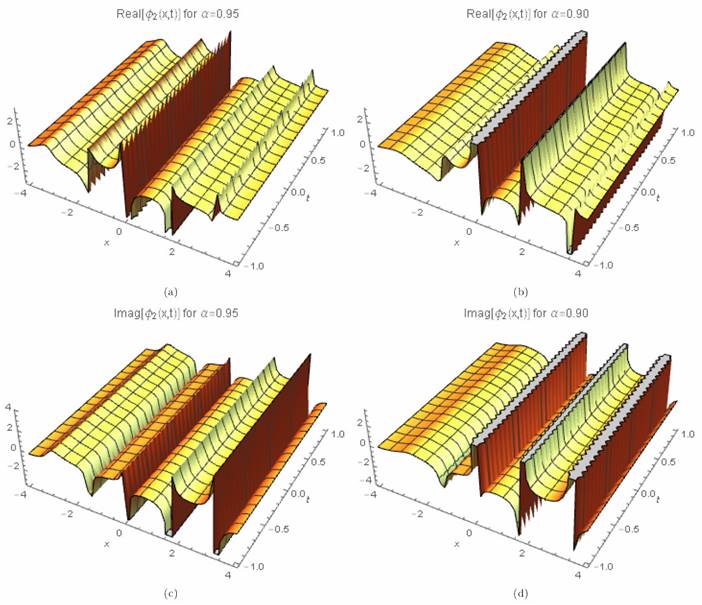
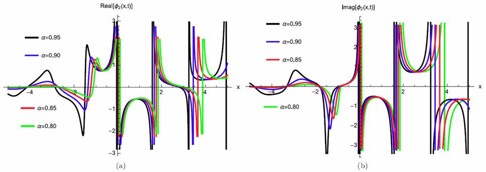
Figure 4 2D Plot soliton solution for Eq. (32) for different particular cases of ρ, arbitrarily chosen.
[Set 3:] We obtain p = [1 - i, 1 + i, 1, 1] and q = [i, -i, i, -i], which gives
We also get
and
Substituting above values into Eqs. (18) and (33), we have
Therefore an exact solution of Eq. (9) is obtained as
where γ (3 λ + 2 θ) > 0 for valid soliton. Figures 5a)-5d) and 6a)-6b) show the soliton surface and the 2D graph for Eq. (39), respectively.
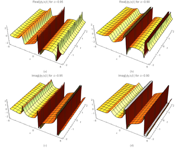
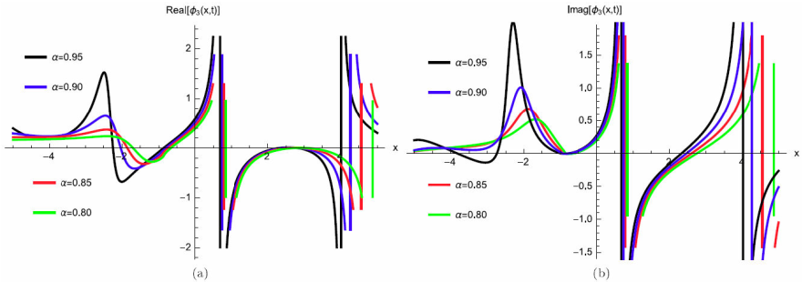
Figure 6 2D Plot soliton solution for Eq. (39) for different particular cases of ρ, arbitrarily chosen.
[Set 4:]
We obtain p = [-1, 0, 1, 1] and q = [0, 0, 1, 0], which gives
We also get
and
Substituting above values into Eqs. (18) and (40), we have
Therefore an exact solution of Eq. (9) is obtained as
where γ (3 λ + 2 θ) > 0 for valid soliton. Figures 7a)-7d) and 8a)-8b) show the periodic wave surface and the 2D graph for Eq. (46), respectively.
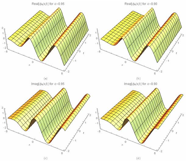
Figure 7 3D periodic wave solution for Eq. (46) for different particular cases of ρ, arbitrarily chosen.
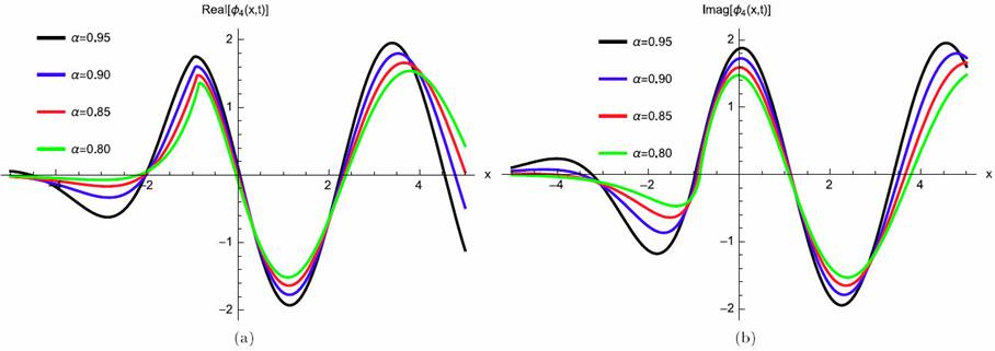
Figure 8 2D Plot periodic wave solution for Eq. (46) for different particular cases of ρ, arbitrarily chosen.
[Set 5:] We obtain p = [-3, -1, -1, 1] and q = [-1, 1, -1, 1], which gives
We also get
and
Substituting above values into Eqs. (18) and (47), we have
Therefore an exact solution of Eq. (9) is obtained as
where γ (3 λ + 2 θ) > 0 for valid soliton. Figures 9a)-9d) and 10a)-10b) show the periodic wave surface and the 2D graph for Eq. (53), respectively.
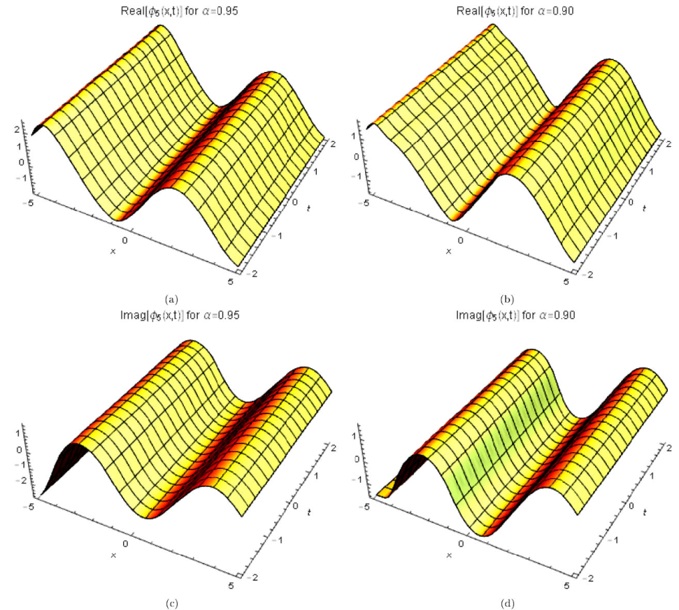
Figure 9 3D periodic wave solution for Eq. (53) for different particular cases of ρ, arbitrarily chosen.
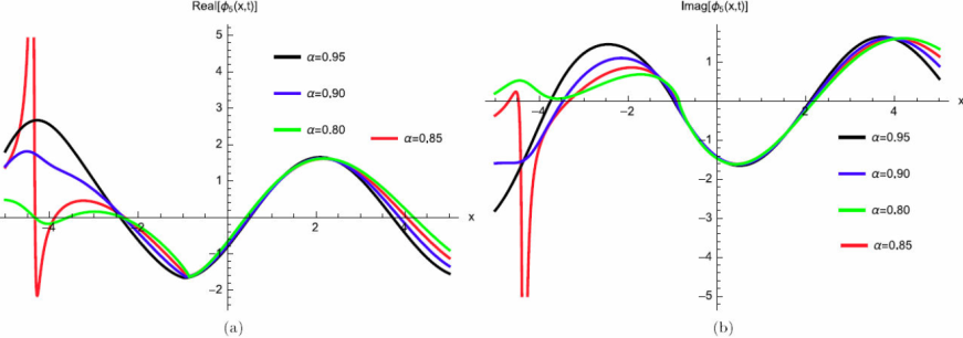
Figure 10 2D Plot periodic wave solution for Eq. (53) for different particular cases of ρ, arbitrarily chosen.
[Set 6:] We obtain p = [1 - i, 1 + i, 1, 1] and q = [-i, i, -i, i], which gives
We also get
and
Substituting above values into Eqs. (18) and (54), we have
Therefore an exact solution of Eq. (9) is obtained as
where γ (3 λ + 2 θ) > 0 for valid soliton. Figures 11a)-11d) and 12a)-12b) show the periodic wave surface and the 2D graph for Eq. (60), respectively.
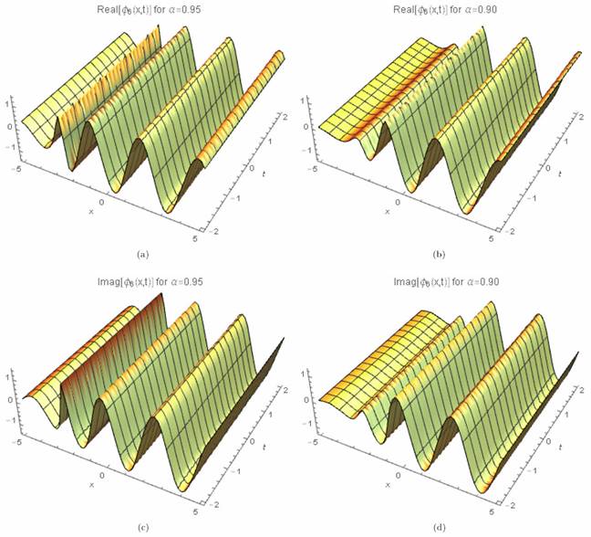
Figure 11 3D periodic wave solution for Eq. (60) for different particular cases of ρ, arbitrarily chosen.
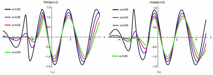
Figure 12 2D Plot periodic wave solution for Eq. (60) for different particular cases of ρ, arbitrarily chosen.
[Set 7:] We obtain p = [2, 0, 1, -1] and q = [1, 0, 1, -1], which gives
We also get
and
Substituting above values into Eqs. (18) and (61), we have
Therefore an exact solution of Eq. (9) is obtained as
where γ (3 λ + 2 θ) > 0 for valid soliton. Figures 13a)-13d) and 14a)-14b) show the soliton surface and the 2D graph for Eq. (67), respectively.
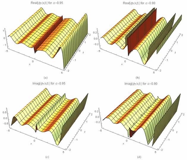
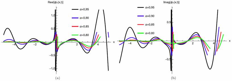
Figure 14 2D Plot soliton surface for Eq. (67) for different particular cases of ρ, arbitrarily chosen.
4. Results and discussion
We discuss the results to Eq. (9) obtained by using the generalized exponential rational function method. As a result, we get new form of solitary traveling wave solutions for this model including novel soliton, traveling waves and kink-type solutions with complex structures. In this work, by using the GERFM, we successfully constructed some exponential and rational function solutions to Eq. (9). When we compare our results with the results reported in [40-47], we observed that, all the results obtained in this study by using the above method are newly structured solutions. These soliton solutions are located throughout parameter restrictions that provide their existence and novel soliton, traveling waves and kink-type solutions with complex structures while other solutions that emerged from the Laplace-Adomian decomposition method, traveling wave hypothesis, extended trial function scheme, among others. These soliton solutions are being reported for the first time in this paper. It shows that the GERFM give an effective and credible mathematical tool for various nonlinear evolution equations to obtain a variety of wave solutions. All solutions are satisfied with their corresponding original equations.
5. Conclusion
In this work, we have obtain exact analytical solutions including novel soliton, traveling waves and kink-type solutions with complex structures for the perturbed β-conformable-time Radhakrishnan-Kundu-Lakshmanan equation. The generalized exponential rational function method is successfully applied to obtain soliton solutions. It is worth mentioning that whole solutions of φ 1 - φ 9 in this article are new and being reported for the first time. From our results obtained in this paper, we conclude that the generalized exponential rational function method is powerful, effective and convenient for the analysis of nonlinear conformable-time partial differential equations involving β-conformable derivative. The obtained results may be utilized to understand the certain physical phenomenons in science and engineering in general and in fiber optics in particular.

