1. Introduction

Trajectories of a charged particle moving under the influence of a magnetic field on any Riemannian manifold are represented by magnetic curves. A magnetic field on a k-dimensional Riemannian manifold (𝓡,○) is any closed 2-form 𝓖. The Lorentz force of the magnetic field 𝓖 is a one-to-one tensor field Ψ such that it is defined by

Ψ (A) ○ B = G (A, B) ; where ∀ A, B ∈X R.

Magnetic trajectories of the magnetic field 𝓖 correspond to magnetic curves δ on 𝓡. These curves satisfy the following Lorentz formula

Evidently, magnetic curves generalize geodesics due to the following equation, which is satisfied by geodesics:

This formula obviously represents the Lorentz formula in the nonappearance of the magnetic field. Consequently, a geodesic corresponds to trajectory of the moving charged particle when it is free from any magnetic field (𝓖 =0) [¹].

In the case of a 3D Riemannian manifold (𝓡,○), vector fields and 2-forms can be described thanks to the volume form dv _h and the Hodge star operator ★ of the manifold. Hence, divergence-free vector fields and magnetic fields are in (1−1) correspondence. Therefore, Lorentz formula is given for any vector field S on the 3D Riemannian manifold as follows:

where 𝓖 is a magnetic field such that ∀S ∈ X(𝓡) with div(𝓖) = 0. As a consequence, the magnetic flow reduced by the Lorentz formula is written by the following form

In three-dimensional Riemannian and pseudo-Riemannian manifolds, this fact leads to describe several class of magnetic curves including Killing magnetic curves and Killing magnetic fields [²,³]. Another classical model of magnetic fields is easily developed if one multiplies by a magnitude the area of a Riemannian surface. Thus, it is obtained that on a hyperbolic plane ℍ² magnetic trajectories are either open curves or closed curves, on the Euclidean plane magnetic trajectories are circles, and on the sphere 𝕊² they are tiny circles having a particular radius [⁴,⁵]. Studies on magnetic curves have been mainly focused on the charged particle, which is assumed to be free of any external force. However, in this manuscript, we consider a well-known external force and attempt to observe its effects on the motion of the charged particle lying fully on the unit 2-sphere 𝕊².

In this manuscript, we take the unit sphere 𝕊² and the transformation δ: 𝕀 → 𝕊² ⊂ ℝ³ Even though the selection of the spherical frame is basically owing to its geometrical understanding, it may be seen that the features of the trajectory of the particle frequently emerge in physics. Considering the definition of 𝕊2 and δ in terms of the orthonormal frame together with the specially defined dynamical force fields, we firstly define a special magnetic curve, which is named as a spherical frictional magnetic curve (𝕊𝑓 −magnetic curve) of spherical vector fields. After presenting its geometric interpretations, we investigate the magnetic and electromagnetic field effects on the magnetic trajectories of the 𝕊𝑓-magnetic curve on the 𝕊².

2. Geometric Background of a Curve on the Sphere 𝕊²

The geometric characterization of curves is a very efficient method to comprehend many physical events. Through connecting with the motion of the particle in a given spacetime, these physical events have been modeled by the geometric equivalences.

Ordinary space is one of best fitted geometric settings for many physical phenomena such that it has been intensively studied by both differential geometers and physicists. Since the unit sphere 𝕊² is a submanifold of the ordinary 3-space we firstly give geometry of the curves in the ordinary 3-space.

Ordinary 3-space is a vector space endowed with a standard metric

x ○ y = x ₁ y ₁ + x ₂ y ₂ + x ₃ y ₃ ,

where x = (x _1, x ₂ , x ₃) , y = (y ₁ , y ₂ , y ₃) are arbitrary vectors in the space: The norm function of the given vector x is defined by ǁxǁ = (ǀx ○ xǀ) ^1/2 and x is called a unit speed or an arc-length parametrized if ǁxǁ = 1.

Now, we can define the unit sphere 𝕊², which is the analogue of the ordinary 3-space, by using the argument discussed above in the following manner:

Hereafter, we consider a smooth regular curve lying fully on the 𝕊² . In the theory of curves, one of the most efficient ways of exploring the intrinsic feature of the curve is to consider its orthonormal frame. It is constructed by a number of orthonormal vectors and associated curvatures depending on the dimension of the space. For the case of 𝕊² , this orthonormal frame was introduced by Koenderink and O’Neil [⁶,⁷]. The curve satisfying the spherical frame equation is called a spherical curve. Finally, we are ready to establish the orthonormal frame of spherical curves lying fully on the 𝕊².

Let δ : 𝕀 → 𝕊² be a unit speed regular spherical curve, that is it is an arc-length parametrized and sufficiently smooth. Then the spherical frame is defined along the curve δ as follows:

Where ∇ is a Levi-Civita connection and µ = det (δ,T,T’) is the geodesic curvature of δ. The following identities including pseudo vector product also hold [⁸]:

δ = T × N, T = N × δ, N = δ × T.

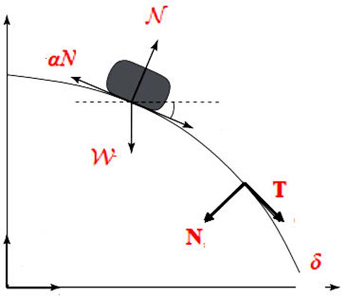
The problem on the motion of the particle on a block or on a surface is well-known and it is extensively studied for the cases of circular and flat surfaces. Point particle sliding on a downward concave surface under the action of a frictional force, a normal force, or a gravitational force can be expressed by using the orthonormal frame, which is defined along the trajectory of the point particle. It is shown that for any particle sliding down on a surface with a mass m, the normal force is

where N = ǁ𝓝ǁ ; the gravitational force is

where g _i =0,1 are gravitational coefficients; the frictional force is

where α is a frictional coefficient [⁹]. These forces and the trajectory of the particle on the section of the 𝕊² can be seen in Fig. 1.

Figure 1 Particle trajectory together with the force fields. 

3. Magnetic Fields of 𝕊𝑓-magnetic curves on the Unit Sphere 𝕊²

In flat spacetime, the motion of a charged point particle was highly active and popular research field since the early study of Poincare, Abrahams, and Lorentz. As such, Einstein’s study of special relativity was inspired on the electrodynamics of moving objects. Poincare and Lorentz were also motivated and guided by the equations of Maxwell to investigate spacetime transformations. This gave rise to the radical unification of some special spacetime structures. In this context, it is fairly true that Maxwell equations played a key role to comprehend the profound connection between the dynamics of the major physical fields and interactions. Further researches, in turn, led to connect the spacetime geometry with the electromagnetic field. As a conclusion, one reaches that the field equations are entirely general at the very base of electromagnetic theory, regardless of considering of any affine structure or metric of spacetime, however, its comprehension in spacetime by way of essential connections, admits constitutive relations between the causal framework of spacetime and electrodynamics.

In this section, we attempt to explore the impacts of Riemannian geometry on the motion of a spherical charged particle under the influence of some external force fields acting on a magnetic field derived from generalized Lorentz equations. Followings are also useful sources to understand the background of the study. Dynamics of the charged particles that correspond to the trajectories of a particular type of curves in electromagnetic fields has been of significance in the literature and it is applied to many experimental studies [¹⁰-¹³]. Furthermore [¹⁴,¹⁵] studied the motion of charged particles in homogeneous electromagnetic fields by concentrating on the invariant geometric description of their trajectories. Bearing in mind, the importance of the frictional force of the dis-placement of charged particles in magnetic fields, Coronel-Escamilla et al. [¹⁶] focused on the fractional dynamics of charged particles in harmonic magnetic fields, ramp magnetic fields, and constant magnetic fields. Körpınar and Demirkol also defined frictional and gravitational magnetic curves together with their energy functionals and uniformity conditions on the 3D Riemannian surface [¹⁷,¹⁸].

Here, we assume that β is a moving spherical charged particle with a magnetic field 𝓖 such that it is influenced by the frictional force on the unit sphere 𝕊² . We also assume for the rest of the manuscript that the trajectory of this particle corresponds to a unit speed sufficiently smooth regular spherical curve δ : 𝕀 → 𝕊² to define and investigate frictional spherical magnetic curves lying fully on the unit 2-sphere by using the spherical orthonormal frame describing along with the trajectory.

Definition 1. Let β be a moving spherical charged particle under the influence of a frictional force in the magnetic field 𝓖 on the 𝕊² such that its trajectory corresponds to a unit speed sufficiently smooth regular spherical curve δ : 𝕀 → 𝕊² . Frictional spherical magnetic trajectories (𝕊𝑓-magnetic curve) of the charged particle β are defined via the Lorentz force formula as follows:

Proposition 2. Let δ be an arc-length parametrized frictional spherical magnetic curve together with the spherical frame elements {δ T, N, μ} on the unit sphere 𝕊² . Then, Lorentz force Ψ of the magnetic field 𝓖 is written in the spherical frame as follows:

where c is an arbitrary smooth function along with the magnetic curve such that it satisfies c = Ψ(N) ○ δ

Proof. Let δ be an arc-length parametrized 𝕊𝑓-magnetic curve on the 𝕊² together with the spherical frame elements{δ, T, N, µ}. One knows that

{Ψ (δ), Ψ (T), Ψ (N)}∈ span {δ, T, N}.

From the definition of the 𝕊𝑓-magnetic curve given in the Eq. (8) together with the spherical frame equations given in the Eq. (4) and the frictional force in the Eq. (7), one has

Ψ (f) = (αN) δ−(αN)’ T−(αNµ) N.

If one also considers the following feature of the Lorentz force tensor field Ψ

Ψ (f) ○ δ = − f ○ Ψ (δ),

Ψ (f) ○ T = − f ○ Ψ (T),

Ψ (f) ○ N = − f ○ Ψ (N),

then it is obtained following equalities:

αN = Ψ(f) ○ δ = − f ○ Ψ(δ) = αN(T ○ Ψ(δ)),

− (αN)’ = Ψ(f) ○ T = −f ○ Ψ (T) = αN(T ○ Ψ (T)),

− αNµ = Ψ (f) ○ N = −f ○ Ψ (N) = αN(T ○ Ψ (N)).

Finally, using the obvious properties of the inner product one has

where c _i (i = 1,...,6) are smooth functions along with the 𝕊𝑓-magnetic curve. Here if one also uses the antisymmetric feature of the Lorentz force

Ψ(T) ○ T = Ψ(N) ○ N = Ψ(δ) ○ δ= 0

and following identities

Ψ (δ) ○ T = −δ ○ Ψ(T),

Ψ (δ) ○ N = −δ ○ Ψ(N),

Ψ (T) ○ N = −T ○ Ψ(N),

then it is concluded that

c ₁ = − (αN)’/αN = c ₆ = 0,

c ₃ = − 1, c ₄ = µ, c ₅ = −c ₂ = c.

If one plugs each value obtained in the Eq. (11) into the Eq. (10), then the proof is completed.

This proposition proves that the Lorentz force Ψ in the spherical frame of the 𝕊𝑓-magnetic curve and the T−magnetic curve on the 𝕊² is the same. Some characterizations of the T−magnetic curve on the 𝕊² have been given by Abdel-Aziz et al. [⁸]. In particular, they find a magnetic vector field 𝓖 as the trajectory of the T−magnetic curve on the 𝕊². Thus, we can apply their finding to our case and give the following theorem due to the similarity of the Lorentz force Ψ in the spherical frame of the 𝕊𝑓-magnetic curve and the T−magnetic curve on the 𝕊².

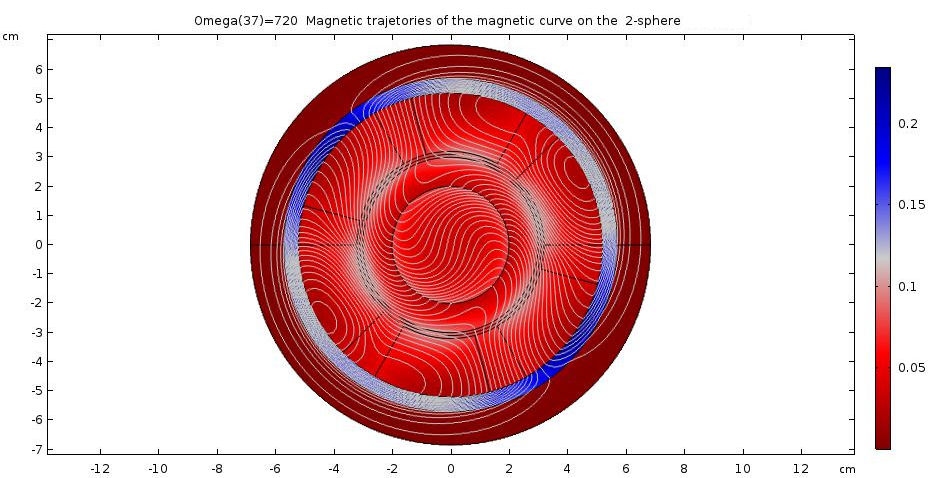
Theorem 3. δ is a unit speed 𝕊𝑓-magnetic curve of the magnetic field 𝓖 if and only if

along with the Sf-magnetic curve, where c = Ψ(N) ○ δ and (αN)’ = 0 [⁸]. Figure 2 demonstrates the magnetic trajectories of the 𝕊𝑓−magnetic curve on the unit sphere 𝕊². It is used the charged particle tracing module of Comsol Multiphysics software to create this sample demonstration.

Figure 2 Magnetic trajectories of the 𝕊𝑓- magnetic curve. 

4. Magnetic Motion of the β on the Unit Sphere 𝕊²

In this section, we define the non-relativistic magnetic motion for the spherical charged particle β with a charge q and mass m, which acts under the frictional force, in the presence of magnetic field 𝓖 on the 𝕊² . The Newton second law for the Lorentz force is readily computed by

where T is the velocity vector [¹⁹]. If one considers Eqs. (4,12,13), then it is obtained that charge to mass ratio of the β on the 𝕊² is equal to -1. The ratio of the charge to mass is intensely used in the electrodynamics of the charged particles particularly in electron optics, cathode ray tubes, electron microscopy, accelerator, nuclear physics, and mass spectrometry. The significance of the ratio of charge to mass regarding electrodynamics is released on the fact that two particles having the same ratio move in the same trajectory in a vacuum when they are subjected to the magnetic fields. However, we rather choose to focus on some mathematical equalities including this ratio to obtain new characterizations for 𝕊𝑓-magnetic curves.

It is known that the magnetic force causes the centripetal force, thus cyclotron radius or gyroradius r is described by the radius of the curvature of the trajectory of the unit speed magnetic curve whose charge is q; mass is m; speed is v; and the strength of the magnetic field is G as the following equality:

In this case, since the ratio of charge to mass is -1, the radius of gyration and the gyro-frequency of the 𝕊??-magnetic curve are computed respectively as follows:

where μ is the geodesic curvature of δ and c = Ψ(N) ○ δ. In the theory of a classical electromagnetism, Larmor theorem states that a rotating charged particle has a magnetic moment such that it is proportional to its angular momentum. Thus, we can present the following consequences.

The angular momentum or mechanical angular momentum of the β on the 𝕊² is given by

Here, one can easily induce that the magnitude of the angular momentum of the β on the 𝕊² is

There also exists another expression for the magnitude of the angular momentum (ǁ??ǁ = mvr) that we can take into account to find out the constant function c = Ψ(N) ○ δ in terms of the geodesic curvature μ of the δ and coefficients of the force fields α, N. If one uses that definition together with Eqs. (15,17), it is yielded that

Thus, we get

Finally, we reach to the point where the magnetic moment of the β on the 𝕊² is written as a vector field:

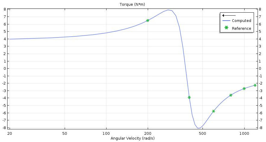
All these results include the behavior of the β on the 𝕊² with spin in a magnetic field 𝓖 on the 𝕊² . Hence, β experiences a torque given by the following identity:

where μ is the geodesic curvature and c = ± (μ ² - 1 + (1= α ⁴ N ⁴ (μ ² + 1))) ^1/2 . In Fig. 3, it is given relation between the angular velocity and magnitude of the torque of the charged particle.

Figure 3 The torque of the β on the 𝕊².  

Now, we are able to investigate the potential energy (𝒫) of the β on the 𝕊² by only using the geometrical coefficients that are presented along with the paper:

Generalization of the angular momentum is constructed by the magnetic force-torque and the mechanical angular momentum:

Gauge invariance is guaranteed due to this structure. If 𝑓 ○ 𝓖 = Ψ(𝑓) ○ 𝓖 = 0; then it is found that c = 0 and

where 𝓖 =µδ−N. As a result, 𝓛 _G and 𝓖 are parallel and it implies that the motion of the β on the 𝕊² is invariant with respect to rotations

Main Result: This approach can also be extended to characterize the torque and the potential energy of each Lorentz force Ψ of the magnetic field 𝓖 on the 𝕊². Namely, if one considers each Lorentz force equation of the spherical frame at the Eq. (9) and following formulae

then it is obtained a magnetic torque of each Lorentz force as follows:

where

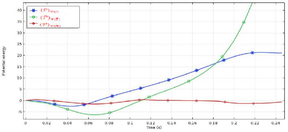
Finally, the potential energy of each Lorentz force Ψ of the magnetic field 𝓖 on the 𝕊² are given by

In Fig. 4, it is shown the variation of the potential energy of each Lorentz force field with respect to time.

Figure 4 The potential energy of Lorentz force Ψ of 𝓖 on the 𝕊2. 

5. Electrodynamics of the β on the Unit Sphere 𝕊²

The fundamental of electrodynamics is constructed upon the theory of Maxwell together with electromagnetic field (EMF), energy, force, and momentum, which are closely connected each other by the Lorentz force law and the theory of the Poynting vector. This theory governs the electromagnetic energy flow and its exchange between magnetic and electric fields. EMF transports both momentum and energy. In this section, we aim to explore the chance of angular momentum being associated with EMF.

Generalizing the Lorentz force law given at the Eq. (13), one obtains that

which is the force exerted on a moving spherical charged particle β with a velocity vector field T in the electromagnetic fields 𝓖 and Ɛ [¹⁹]. If one considers Eqs. (4,12), it is easy to get that

where μ is the geodesic curvature of the curve. Thus, one can compute the Poynting vector 𝒮, which represents the direction of propagation of trajectories of the 𝕊𝑓-magnetic curve on the 𝕊² as well as the density of energy flux. From Eqs. (12,19), one has

where c = Ψ(N) ○ δ: Based on this definition the density of the angular momentum of the EMF is defined by

Thus, the angular momentum of the EMF is defined by

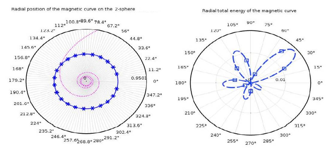
Since EMF also stores energy then we can discuss the energy density of the electromagnetic trajectories of the β on the 𝕊² . The total energy 𝒰 contained in a section of the 𝕊² with both magnetic and electric field is

In Fig. 5, it is seen magnetic trajectories of β under the electromagnetic fields and total energy density on the 𝕊².

Figure 5 Magnetic trajectories and total energy of β on the 𝕊². 

6. Conclusion

The subject of electromagnetic force and optical angular momentum is highly broad and many distinguished research papers, reviews, and monographs have been devoted to these topics for a long time. The aim of the paper has not been to report new discoveries nor to break new ground. Rather, it has been our goal to show how the findings obtained through-out the manuscript are useful and applicable to clarify some of the fundamental features of the electromagnetic force, energy-exchanges rate, optical angular and linear momentum, and optical magnetic-torque experienced by the spherical frictional magnetic curve ( 𝕊𝑓- magnetic curve) of spherical vector fields on the sphere 𝕊² .

It is desired that our meticulous debate of the principles considering the Serret-Frenet law and Lorentz force law in conjunction with a coherent practice of the statement of some special magnetic curves, electromagnetic force, optical angular momentum, torque, magnetic-force torque, has been beneficial in clarifying some of the aspect of the spherical charged particle in a continuous motion with a magnetic field on the sphere 𝕊² while it is exposed to a frictional force, on the unit sphere 𝕊² .

This study will also lead up to further research on the investigation of the electrodynamics of the moving spherical charged particles when they are experienced some other well-known external forces beside the the frictional force such as the gravitational force, the normal force, and the resultant force. Consequently, we aim to obtain more applicable and widely acceptable results to comprehend the exact movement of the spherical charged particle in a given geometric and physical spacetime structure.