


 nueva página del texto (beta)
 Inglés (pdf)
 Artículo en XML
 Referencias del artículo
 Enviar artículo por email
 Citado por SciELO
  Similares en
SciELO
Similares en
SciELO 
 Permalink
1. Introduction
For many years, several models about tide generation have been realized using the basic knowledge of mechanics [1,2], and these approximations are based on the gravitational interaction of the Moon and the Sun with the Earth. Also, there is another elegant and complex formalism to model this interaction [3]. In the same sense, there are not analytical equations to predict the tide in coasts, bays, lakes and estuaries; where the height h is normally amplified. This is due to the strong dependence on the shape of their soil layers and the narrowing of their cavities [4].
On the other hand, the experimental determination of the tide height is typically carried out with tide gauges or mareographs. Several devices have been developed for this purpose including graduated rules, manometer gauges, satellite measurements [5], accelerometers systems [6], microwave interferometers [7] and ultrasonic devices [8]. This last kind of tide meters takes advantage of the versatility of the ultrasonic transducers, to carry out the liquid volume monitored. At this respect, several works describe low cost devices to automatically determine and control the liquid level in a container without contact and using Arduino technology [9-12]. In this work, two identical cheap homemade prototypes are built to determine the tide height in places near coasts and they are based in ultrasonic signals detection.
The main aim of this work is to compare the measurements of h with the simplified model of oceanic tides and then to determine the tide amplification effect in the mouth of the Serinhaém estuary.
2. Theoretical Background
Assuming the Moon and the Sun as static spheres and the water deformation as ellipsoids [1,2,13], at any time, the oceanic tide height H can be calculated using the following Eq. (1a). Here, Mm and Ms are the masses of the Moon and the Sun; rm and rs are the distances from the center of the Moon and the Sun to the Earth’s surface, respectively; M e and R are the mass and radius of the Earth. Then, there are two induced ellipsoidal deformations, which are caused by the Moon (Hm) and the Sun (Hs), respectively. Analyzing the Moon displacement θm displayed in Fig. 1(A) and assuming a similar configuration for the Sun displacement θs, the minimum values of H are reached at θm = θs = π=2,/ 3π/2 (at the first and third quarter of the moon period), which happens when the semi-major axis of both ellipsoids are orthogonal as is shown in Fig. 1(B). The maximum H occurs when they are parallels, i.e., θm = θs = 0; … (full and new moon, respectively) (Fig. 1(C)).
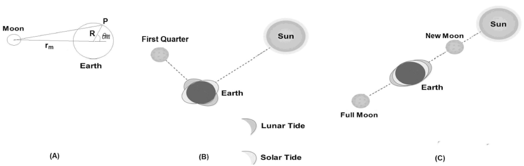
Figure 1 (A) Free body diagram of the Moon-Earth system separated for rm, (B) the first quarter of the lunar phase and (C) the new and full moon phase.
Due to the sinusoidal dependence over time, the maximum total expected tide height h for oceanic water is computed as the difference between maximum and minimum H values (h = H max -H min) [1,2], given by Eqs. (1b) and (1c). Hence, substituting the next values [14]: M m = 7.35 × 10²² Kg, M s = 1.98 × 1030 Kg, M e = 5.98 × 1024 Kg, rm = 384 × 106 m, rs = 150 × 109 m and R = 6.37 × 10⁶ m, it is approximately estimated that h = 54 + 24 = 78 cm. In fact, this is the sum of the peak to peak amplitudes of Hm and Hs. Now, if we considered the spin motion of the Earth (with angular velocity ω = 2π=P , where P = 24 h 22 min) plus its precession displacement δ around the z axis (δ m and δ s are relative to the Moon and the Sun precessions respectively). Thus, in a point on its surface placed with latitude λ and longitude φ, the Eq. (1a) must be replaced by Eq. 1(d) [2]. With this equation are modeled the two increasing and decreasing sinusoidal tides, which are produced in a day approximately, they are called high-tide and low-tide respectively.
An example where the approximation of Eq. (1a-d) dramatically fails is the Fundy bay in Canada, where h reaches up to 20 m [15]. This amplifying phenomenon (like a water gain) is caused by the superposition of the periodic propagation/reflections of water on the coast borders, which reach up to a hydrological resonance in some cavities.
On the other hand, in geophysics an estuary is defined as a partially enclosed coastal body in the ocean with at least a river flowing into it and an extreme (called estuary mouth) connected to an ocean. The closed extreme is called estuary head [16]. Physically, the estuary could be seen as an irregular cavity where water currents are periodically propagated.
Regarding the previously mentioned amplifying effect of the tide near coasts, we defined the tide gain G in an estuary as the ratio between the peak to peak amplitude A pp of tide at a point near to the estuary head (Ah pp ) in relation to the App value in the estuary mouth (Am pp ), given by Eq. (2). This definition could explain the relation G ≥ 1, because the tide behavior in the estuary mouth is more similar to that of the ocean tide.
3. Materials and methods
The development of this system (called TidalDuino) is realized with the help of Arduino boards and ultrasonic sensors (transmitter plus receiver) and works as a data logger for a long period of time. This apparatus is calibrated in our physics lab by way of controlled experiments to determine distances via ultrasonic waves, which were simulated under established controlled conditions. TidalDuino sends an ultrasonic wave with velocity vs (340 m/s in the air), which later is reflected to the starting point (after a time T o F) by an obstacle placed at distance d, then it ideally satisfied Eq. (3).
As v s in air depends on its temperature and humidity [17-19], it must be replaced for the corrected speed of sound v sc , given by Eq. (4) in ms -1 units, which includes the air temperature T in ° C. The v sc allows higher fidelity with regard to the distance estimation of obstacles located in a medium with variable temperature.
In Fig. 2, the block diagram of TidalDuino in operation on an estuary segment is displayed. As is observed, the device is subject to a metallic support; also, the Arduino UNO board is the main piece including an ATmega328 microcontroller. The board is connected to different peripherals of hardware blocks: a real time clock integrated circuit DS1307, flash memory of 2 GB, ultrasonic transmitter/receiver HC-SR04, temperature sensor LM35, battery bank 12V/9A, and a PC with display, which is optional because the system is able to work autonomously. The HC-SR04 transducer operates through piezoelectric effect using ultrasonic pulses to determine the distance to the water surface h ws by adapting the called time of flight method. For this purpose, when a trigger signal provided by the ATmega328 excites the transmitter during 10 μs, it sends a sequence of ultrasonic pulses of 40 kHz through the air. If the waves are reflected (echo) by the water, this reflection is detected by the receiver in the echo terminal as a rectangular pulse. Thus, a digital input of the microcontroller will shift to a HIGH state during time t = T o F. Then, the air temperature is obtained to estimate v sc and the left side of Eq. (3), within the microcontroller. At the same time, the date and time are recorded by the DS1307. Hence, the elapsed time plus its corresponding h ws are written in an electronic text file and stored in a flash memory for offline analysis.
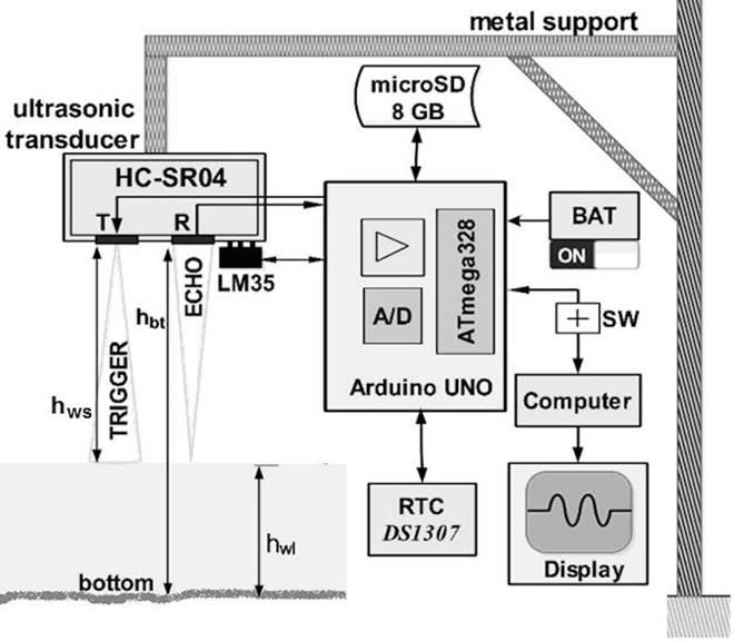
Figure 2 Block diagram of TidalDuino in operation on an estuary segment, with the HCSR04 sensor fixed in a metallic support from a distance h bt to the estuary bottom.
To increase the reproducibility of this device, the hard-ware scheme and the electrical connections between the Arduino UNO board and the different analog/digital peripherals circuits and sensors are specified in Fig. 3, which is a very similar electronic circuit that the used in [9]. Specifically, it is observed that the LM35 sensor output (central pin) is connected to the analog input A0, and according to the manufacturer’s specifications, the relationship for conversion is 10 mV per ° C. Meanwhile, the trigger and echo terminals of HCSR04 are connected to (DIO7) and (DIO8), respectively. The former is configured as digital output and the latter as digital input. In addition, as is observed in the bottom of Fig. 3, the SCL and SDA terminals of the integrated circuit DS1307 are connected to A4 and A5 analog inputs. This circuit is powered by another battery of 3.3 V and is also complemented with a 32.768 kHz quartz clock to transmit the data and hour to the Arduino board. The complete code for automation can be freely downloaded from the following electronic address: http://dfisweb.uefs.br/tide/tide.rar.
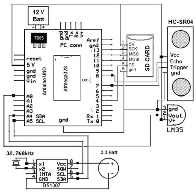
Figure 3 Schematic diagram of Arduino UNO board connected with HC-SR04 and LM35 sensors, also the DS1307 clock and SD card, powered with 12 V batteries but is regulated to 5 V.
3.1. Calibration of TildalDuino
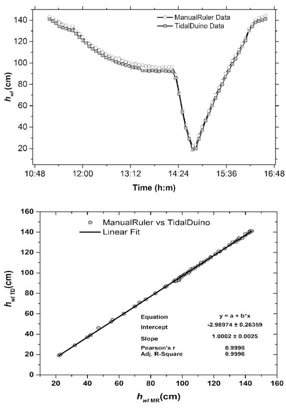
In order to analyze the TidalDuino performance, an experiment is conducted for calibration in the laboratory while maintaining controlled conditions. For this purpose, Tidal-Duino was placed on the top of a water tank attached to a fixed platform, as is displayed in Fig. 4, at a distance h bt from the tank bottom. Indeed, a very similar calibration procedure is performed in [9]. In this figure, the water level h wl was controlled with a system for draining and refilling using a valve. Through this means it is connected with another small container of the same height and a graduated ruler is placed inside, to manually measure h wl . Then, an arbitrary function of the water variation along the time was performed to simulate the tide level, starting at h 0 = 140 cm. Thus, initially h wl was manually set and it is softly diminished each 5 minutes. Later the drain speed is increcresedais increased the drain speed, reaching approximately 20 cm. Finally h wl is lineally increased up to 142 cm. In this experiment, h wl was directly measured using the ruler (h wlMR ) and it was simultaneously estimated applying Eq. (5) with TidalDuino (h wlTD ).
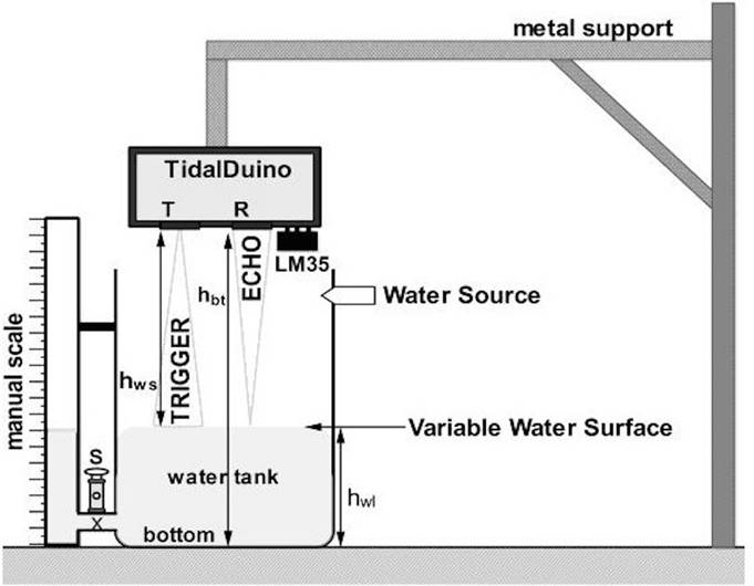
Figure 4 Schemes of the calibration experiment measuring the water level simulating the tide motion, respectively.
In Fig. 5(A), the experimental results of h wl are displayed. The maximum observed discrepancies do not exceed 3 cm, and they are always observed at the time when h wl is diminishing between the hours 14:30 and 15:00, due to the quick water level diminution in this interval. In contrast, when h wl increased, the maximum discrepancy was less than 2 cm. It is important to emphasize that the observed discrepancies in this experiment were due to instability of the water surface; this was more evident when the water escaped to the draining deposit. Other spurious uncertainties could have been due to the surface curvature of water. In Fig. 5 (B), the correlation between h wlMR and h wlT D is shown. With the help of a simple analysis using fitting straight line, it could be concluded that this device exhibits a slope m = 1.000±0.003 with a Pearson coefficient of 0.999, confirming the linear performance of TidalDuino and improving the correlation parameters reached in [9].
4. Experimental results and discussions
After calibrations, TidalDuino was ready to work in situ, and the chosen place was the Serinhaém estuary situated in Ecopolo III APA do Pratigi (Environmental Protection Area, Portuguese acronym) in the lower South of Bahia State, about 110 km from the state capital, Salvador. In Fig. 6, the map of Serinhaém estuary is shown as well as its close-up view, indicating its geographical localization between parallels 13 ° 30’ and 14 ° 00’ S latitude, and meridians 38 ° 50’ and 39 ° 40’ W longitude.
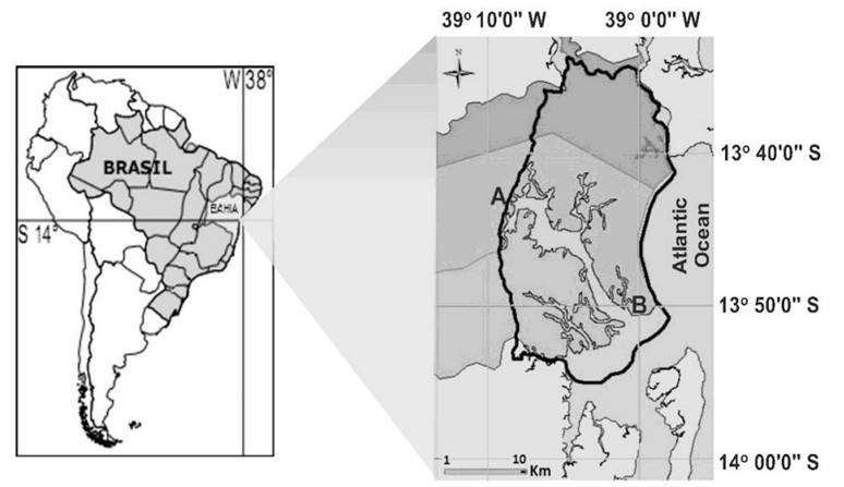
Figure 6 Map of the study site Serinhaém estuary, situated in Ecopolo III of APA do Pratigi, Bahia State, Brazil. On the right is shown a close up view with the point A is the estuary head and B estuary mouth.
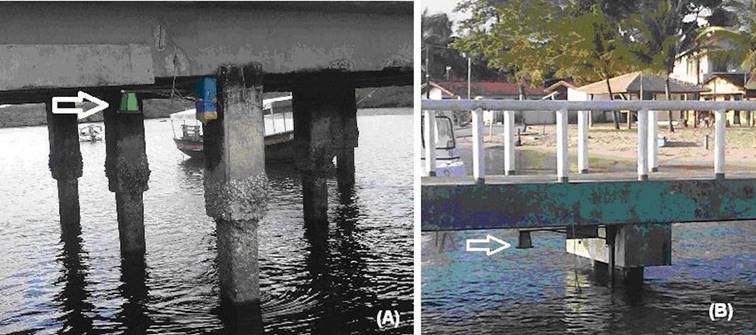
The first TidalDuino was placed at the point A on the pier of Ituberá (estuary head with GPS coordinates 13 ° 44’ 9.7188” S and 39 ° 8’ 47.6304” W) and the other at B, located on the pier of the Barra do Serinhaém (estuary mouth with GPS coordinates 13 ° 50’ 40.902” S and 39 ° 0’ 34.938” W), which disembogues info with the Atlantic Ocean. Both points were separated by 29.5 km and in Fig. 7(A) and (B), the images of the installed devices in each pier are shown.
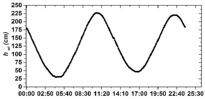
An initial test in situ was carried out on point A over 24 hours. Then, the initial h bt was measured with a graduated tide-rule of 4.5 m long, and this value was introduced to TidalDuino as initial parameter corresponding to the initial time 00:00 hours. The system was programmed to measure hws and then to compute and store the mean value of h wl every 5 min. In Fig. 8, this measurement is displayed, showing the expected sinusoidal behavior and exhibiting two undulations with peak to peak amplitudes of 1.98 m and 1.74 m. Other important observations are a spurious artifact that occurred at 13.15 min of operation and a clear flat trend in the two minimum values and in the second maximum value, indicating no significant differences in h wl along of approximately 45 - 60 min.
In the final experiments, the acquisition and storing of h wl increased to 15 min. Hence, the measurements were simultaneously carried out at both points A and B during September 12 - 17, 2015, in the new moon phase. In Fig. 9 (A), the stored measurements are plotted. In this case, two deformed triangular-like waveforms were obtained, despite the Fig. 8 is sinusoidal. As was observed, few spurious measurements or artifacts are introduced. Indeed, the big artifact observed at point A (after 18 hours of operation) was due to an induced delay in the transmitter/receiver system to replace a power battery. However, during that period the real time clock continues working. In the same way as Fig. 8, again a flat behavior on the peaks of the deformed triangular shapes is evidenced in a zoomed view of Fig. 9(B), indicating non-significant differences in h wl during 45 - 60 min. Although the shape of the signals was deformed triangles, which is unexpected by comparing with Fig. 8 and the theoretical models, this effect is due to the diminution of the sampling frequency and the centimeters resolution of the system (1 cm). Nevertheless, it is expected that the parameters of period and amplitude do not differ from the corresponding sinusoidal shape, because we are sampling 24 times more than the limit established by the Nyquist-Shannon sampling theorem [20].
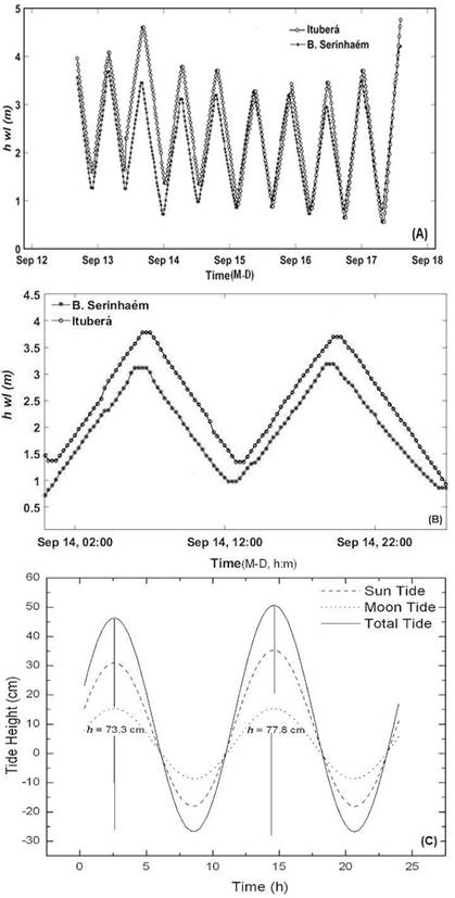
Figure 9 Temporal behavior of h wl measured simultaneously in both piers, (A) over the period September 12 - 17 of 2015, and (B) zoom view of the deformed triangular waveforms; (C) the theoret
In Fig. 9 (C), the computed tide height through the dynamic model (Eq. (1d)) is displayed. In both geographical points, the approximated latitude (λ ≈ 13 ° ) and longitude (φ ≈ 39 ° ) of the GPS coordinates are used, whereas the constant precession of the Moon is δm = 5.14. Although the precession of the Sun is variable, this value is approximated to δs ≈ 0 due the closeness (September 23) of the spring equinox. By means of a quick analysis of this last graph, the mean peak to peak amplitude h = 75.5 cm is estimated, this is less than 3% with the static finding of 78 cm, using Eq. (1c).
Following the discussion of these experiments, the presence of two high and low tides daily was verified at both sites. Also, an almost systematic increase in h wl was observed at the estuary head. The average values of the peak to peak amplitude in the estuary head < Ah pp >= 2.76±0.59 m and the estuary mouth < Am pp > = 2.49 ± 0.49 m were estimated. Both values were calculated by averaging the measurements of Ah pp and Am pp registered every 12 hours. The uncertainties expressed correspond to the standard deviations. Those amplitudes were more than 3 times greater than the h obtained with Eqs. (1b) and (1c). Also, the corresponding average oscillation periods were 12h16’ ± 8.4 and 12h00’ ± 5, respectively. Although two maximum values were observed, the higher determined peak to peak amplitudes (in September 17) are Ah ppmaximum = 4.19 m and Am ppmaximum = 3.74 m, which are more than 4.8 times higher than h. In addition, minimum amplitudes (in September 15) Ah ppminimum = 2.34 m and Am ppminimum = 2.20 m were observed, which were more than 2.8 times higher than h. In the same sense, in Fig. 10 is plotted G vs t using the later values and Eq. (2) and the maximum observed gain is G max = 1.33. This value is reached between September 13 and 14 of 2015, which coincides with the lunar phase where the semi-major axis of both ellipsoidal deformations of water are completely parallels, as is illustrated in Fig. 1(C).
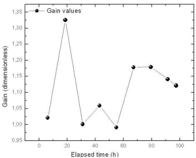
Another observation was the minimum observed gain G = 0.992 after 55 hours of measurement. Thus, in this time, Am was slightly higher than Ah. In addition, it was remarkable that the values Ah ppmaximum and Am ppmaximum were not necessarily related to G max. Moreover, the presence of the last maximum value was contradictory to the described theoretical background. Hence, this phenomenon must have been related to a superposition of water waves in the estuary cavity.
5. Conclusions
In this work, the tide height of the Serinhaém estuary was experimentally analyzed. With the help of two portable home-made remote sensing systems, it was possible determine the tide gain in the estuary mouth. These tide meters were designed to reach a low manufacturing cost, following other experimental setups previously performed to determine liquid levels in open containers. In addition, the calibration parameters obtained are according the reported in these experimental works.
The average tide height determined in the experiments is compared with two simplified theoretical models for oceanic tides. The estimation with static approximation (78 cm) shows discrepancies of 3% approximately, in relation with the dynamic model. Through the analysis of the obtained gains and average amplitudes, a systematic tide amplification effect was corroborated in the estuary head. Also, the discrepancies between the measured amplitudes and the analytical models, showed differences minors than half order of magnitude. Finally, the maximum observed tide gain in the estuary mouth was G = 1.33 approximately and it occurs at the time of the new moon phase. As far as we know, this is the first time that the tide height and gain of the Serinhaém estuary has been experimentally analyzed and compared with an analytical approximation.

