


 nueva página del texto (beta)
 Inglés (pdf)
 Artículo en XML
 Referencias del artículo
 Enviar artículo por email
 Citado por SciELO
  Similares en
SciELO
Similares en
SciELO 
 Permalink
1. Introduction
The monitoring of hazardous elements, such as heavy metals, in superficial water bodies, has become an increasing environmental concern worldwide [1]. Heavy metals are especially harmful due to their bio-accumulation in biotic systems as well as the serious risks they entail for human health [2]. Despite heavy metals are commonly found in the environment at trace amounts (i.e. up to a few ppm) since they are natural components of the Earth’s crust, they can become toxic at higher concentrations. The concentration levels of heavy metals in the environment can be elevated as a result of different main sources: agricultural and industrial activities, sewage sludge spills, and urban/vehicle emissions [3,4].
Some metals, such as Pb, Co, As, and Cd, are extremely hazardous even at very low concentrations. In turn, for others the potential adverse effects on the human body and the environment depend not only on their concentration, but also on several factors including, the dose, route of exposure, and chemical species. Moreover, the age, gender, genetics, and nutritional status of exposed individuals are determinant. For instance, metals such as Cr, Cu, Ni, and Zn are essential trace nutrients that are necessary for different biochemical and physiological functions of biological systems [5]. On the other hand, they can cause harmful effects at higher concentrations. Particularly, for Cr and Cu there is a very narrow range of concentrations between beneficial and toxic effects [2]. Therefore, monitoring these two metals in the environment is of great relevance as they are associated to urban and industrial untreated wastewater. Cr is extensively used in leather and tannery industries. Despite it exists naturally in several oxidation states, the most common and stable forms are the trivalent [Cr (III)] and the hexavalent [Cr (VI)] species. Most of the Cr released into the environment due to anthropogenic activity occurs in the Cr (VI) form, which is highly toxic and carcinogen [6]. Cu is usually employed in industry and agriculture. It enters the environment mainly through the disposal of Cu-containing wastewater. Human exposure to Cr and Cu is associated to severe health problems including allergic reactions, nose, eyes and mouth irritations, stomachaches, kidney and liver damages, and even death [7].
The heavy metal-polluted residues derived from anthropogenic activities are often released into the environment without a proper treatment. Water bodies such as lakes, rivers, and streams, are the ultimate sink of heavy metals [8]. A reliable diagnostics of contaminated aquatic ecosystems is not straightforward because it requires laborious measurements accounting for spatial and temporal variations of the pollutant concentrations. To overcome this difficulty, an alternative approach is to take advantage of the fact that heavy metals settle down and accumulate in the sediments at the bottom of water bodies [9]. Sediments save a valuable record of the environmental history of their aquatic environment. Thus, they are very useful as environmental indicators for the assessment of heavy metal pollution in natural water [10-13].
The most commonly used analytical techniques for determination of heavy metals in sediments are atomic absorption spectroscopy (AAS) and inductively-coupled plasma atomic emission spectroscopy (ICP-AES) [14-18]. However, these techniques are relatively expensive and require a time consuming pre-treatment of the samples (i.e., acid digestion, dilution). Over the past years, Laser Induced Breakdown Spectroscopy (LIBS) has emerged and established as a valuable analytical technology. LIBS is a laser-based spectroscopic technique for the elemental chemical composition of a wide range of materials, including solids, liquids, and gases [19-21]. LIBS method relies on focusing a high energy pulsed laser inside or on the surface of a sample to create a plasma with the ablated material. Typically, laser induced plasma reaches temperatures of ≈ 1 eV and electronic densities of ≈ 1017 cm -3 . Under these conditions, the mass ablated from the target separates into atomic/ionic components which result excited within the plasma plume and then, as the plasma cools, decay to ground levels with light emission [22]. Each element in the periodic table emits a unique LIBS spectrum given by a set of discrete peaks in the UV-Vis spectral range (200-900 nm). The spectral analysis of the emission lines, which are the “fingerprints” of each element, provides both, qualitative and quantitative information regarding the species present in the sample (i.e. ions, neutral atoms, and simple molecules) assuming that the plasma composition is representative of that previous to the laser ablation (stoichiometric ablation). The LIBS technique has the attractive features of performing fast, in-situ, and multi-element measurements requiring a minimum or no sample preparation. These conditions are not feasible with other conventional techniques and, thus, make LIBS a very promising technique to be integrated to the well-established methods [23].
The most common method to achieve quantitative results in LIBS is the construction of calibration curves with reference samples. Nevertheless, the analysis may be hindered by time plasma evolution, spatial inhomogeneity of the plume, self-absorption of the spectral lines, and matrix effect [24]. Matrix effect is related to both chemical composition, and physical properties of the samples which influence negatively the laser energy coupling with the sample surface leading to variations of the intensities of spectral emission and, thus, to inaccurate compositional results [19].
The recent review by Harmon et. al. [25] summarize the current state-of-the-art on LIBS for the analysis of natural materials, termed “GEOLIBS”, including mineral, rocks, sediments, soils, and fluids. Matrix effect is the main draw-back affecting the accuracy of LIBS analytical results from natural samples [26]. Despite several methods have been successfully employed to compensate its effects, the strong matrix effect in fluvial sediments is very hard to ameliorate due to they usually have a wide variable ranges of moisture and organic matter [27,28] Therefore, reducing the undesirable matrix effect is a critical issue that needs to be further investigated to obtain more reliable quantitative results of this kind of materials.
Most research has been devoted to the determination of heavy metals (i.e. Pb, Cu, Cr, Cd, Ni, Ag, Mo, Zn) in soils matrices, in which the feasibility of LIBS method has been proved, as well as the accordance of the analytical results with those of reference methods, e.g. AAS (see Ref. [29] and ref. therein). In turn, relatively few studies have been carried out regarding the analysis of sediments. For instance, Lazic et al. [30] analyzed heavy metals traces in an Antarctic sediment core. Similarly, Barbini et al. [31] reported the qualitative and quantitative analysis of several heavy metals in marine sediments extracted during the XI Italian Antarctic campaign. In another study, Cuñat et al. [32] used a portable LIBS system to measure in situ traces of Pb in road sediments. In addition, Han et al. [33] analyzed the distribution of Al, Si, K, Ca, Mn, Fe, and Sr in sediment cores from the Arctic Sea. Further, the LIBS analysis of fluvial sediments has been poorly explored and very scarce studies are reported in the pertinent literature. Mekkonen et al. [34] applied LIBS for the analysis of levels of Cr, Mn, and Fe in sediments collected from a polluted river in Ethiopia. The concentrations of these metals were quantitative determined through calibration curves employing several certified reference materials of sediments and soils. The obtained results were compared with those from flame-atomic absorption spectroscopy. Even though certified standards can be quite expensive, some observed discrepancies between LIBS and FAAS (Flame Atomic Absorption Spectrometry) were found that were attributed to the occurrence of matrix effect. Austria Jr. et al. [35] used natural zeolite as an alternative diluent/binder to generate matrix-matched standards for calibration purpose. The proposed method was successfully evaluated for the determination of the contents of Cr, Cu, and Pb in sediments collected from a creek running along mining areas.
In the present work, the LIBS technique was applied for determination of heavy metals in fluvial sediments. The total contents of Cr and Cu were quantified in samples collected from a stream passing through the urban area of Tandil city (Buenos Aires, Argentina). Our main goal was to contribute to the optimization of LIBS analysis through overcoming the strong matrix effect present in sediment samples. To this aim, suitable steps of sample preparation and standard calibration were carried out to achieve accurate quantitative results for heavy metal pollution by anthropogenic activity. The information obtained in this study will be useful to address a rapid reliable assessment of the pollution of aquatic ecosystems. Subsequently, more detailed sampling and analysis can be conducted.
2. Materials and methods
2.1. Study area
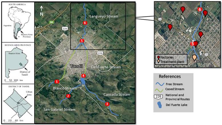
Tandil city (37°19.5’S; 59 ° 08.3’W) is located in the south-east of the Buenos Aires province, Argentina (Fig. 1). It is a medium-size city with an urban area of approximately 50 km2, and a population of 125,000 inhabitants [36]. The Langueyú stream basin begins at the southern of the Tandilia hills belt. Then, two tributary streams, i.e. Blanco and Del Fuerte, run cased through the main urban area and converge to form the Langueyú stream in the north of the city. Here-after, Langueyú stream runs at open air towards the northern receiving a noticeable influence of several anthropogenic activities due to a number of industries settled down in nearby area (see inset in Fig. 1). These include 3 dairies, 1 sausage factory, 1 tannery, and 3 slaughterhouses/refrigerating plants. Also, a domestic sewage treatment plant discharge their liquid effluents into the stream. As a consequence of their productive activities, all these facilities generate wastewater that is discharged directly into the stream. Air pollutant emissions were not detected in the area.
2.2. Sediment samples
The samples employed in this study were fluvial sediments collected upstream and downstream of the Langueyú stream. The sampling design carried out was based on a previous study in which a hydrological analysis of the basin was performed and the main sources that impact directly on the stream were identified [37]. In the mentioned study, a reduced set of 6 strategic sampling points were determined which allowed a rapid hydrological analysis of the whole stream. Therefore, the same selected sites were sampled in this work. The 6 samples (i.e. # 1 to # 6) were collected by using a 1 m - long PVC tube with a diameter of 4 cm in such a way that a shallow sediment core of 5 cm thick was extracted on each case. Samples # 1, # 2, and # 3 were collected from the basing head; sample # 4 from the medium part of the stream; and samples # 5, and # 6 from downstream after the main nearby facilities. At each sampling point, 3 sediment cores were extracted at a depth of 4 cm, which were mixed and well stirred to obtain a single homogenized sample. The collected samples were transported to the laboratory for subsequent LIBS analysis.
All the analytical samples were dried in an oven (at 95 ° C for 6 h) until constant weight, finely ground using a mortar and pestle, and sieved through a #20 840, μm-mesh to remove any coarse elements. After that, the samples were incinerated in a muffle (at 475 ° C for 24 h) to remove their organic and moisture contents. For each sample, 13.5 g of sediment was taken and polyvinyl alcohol (PVA; Merck Schuchardt) was added as binder to improve the sample cohesion while minimizing the matrix effects. We used 0.2 g of PVA in powder form diluted with 2 ml of hot deionized water. Finally, the mixture was stirred, air dried, and pressed in a die (at ≈ 100 MPa for 1 min) to obtain pellets of approximately 3 cm - diameter and 1 cm - thickness.
Following the same procedure, reference samples were manufactured for calibration purposes and for validation of the performance of the LIBS method. The standard addition calibration approach was adopted because it employs the analytical samples itself to avoid changing the matrix of the samples [38]. Unpolluted sediments collected at the sampling point #3 were used. This site was located up in the hills in an area distant from the anthropogenic pollution sources considered in this study, therefore, it was assumed uncontaminated. Reference samples with known Cr and Cu concentrations in the ranges 1-53 ppm and 8-32 ppm, respectively (Table I), were prepared under the standard addition method. The added Cr and Cu solutions were obtained by diluting stock solutions (Cr Standard for AAS, Merck, Germany; Cu Standard for AAS, Fluka Analytical, Switzerland) with appropriate volumes of distilled water.
2.3. Experimental setup
The experimental setup used provided a good spectral resolution that allowed suitable recording of individual line profiles of trace elements with concentrations at ppm levels. It has been used previously [39], so only a brief description is given here. A Nd:YAG laser (Continuum Surelite II, λ= 1064 nm, 7 ns pulse FWHM, 100 mJ/pulse, repetition rate of 2 Hz) was focused at right angle onto the surface of the samples with a lens of 100 mm focal-length to generate the plasmas in air at atmospheric pressure. During the measurements, the pellets were rotated to avoid the formation of a deeper crater by the ablation process, thus improving the reproducibility. The spatially-integrated emission of the plasmas was collected along the line-of-sight in a perpendicular direction to the laser beam by a lens of 200 mm focal-length and focused into the entrance slit (100- μm-wide) of a monochromator (Jovin Yvon Czerny-Turner configuration, resolution 0.01 nm at λ = 300 nm in double passage, focal length 1.5 m, grating of 2400 lines/mm). The emitted light was detected with a photomultiplier (PM, Hamamatsu IP28, spectral response range 200-600 nm) whose signal was time-resolved and averaged with a Box-Car (Stanford Research System). The recorded spectra were processed by a PC using Microcal Origin® software. An accurate wavelength calibration was carried out with a standard Hg pencil lamp. The focused laser spot on the pellets surface was 1.5 mm diameter with a resulting irradiance of about 1 GW/cm2.
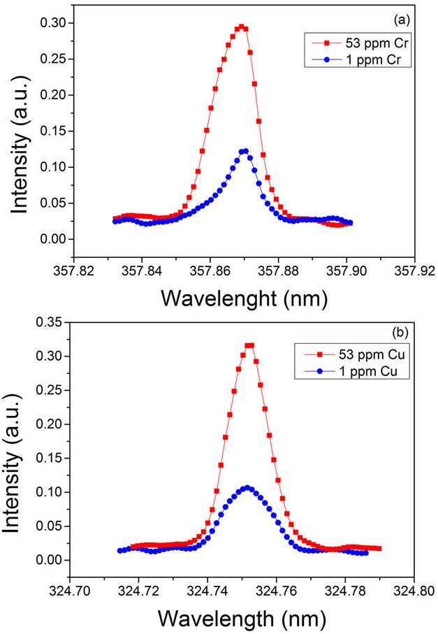
The strong resonant lines Cr I 357.87 nm and Cu I 324.75 nm were selected as analytical lines for quantitative determination of Cr and Cu content in the sediments analyzed. In our experimental conditions, these lines were measured isolated and free from interferences of other elements [40]. The line profiles were measured with a delay time of 8 μs for Cr and of 35 μs for Cu with a fixed gate width of 0.6 μs to discriminate the line emissions from the early plasma continuum. Each point of the emission profile was measured by averaging 3 laser shots, then each spectral line was replicated 3 times and further averaged. In such conditions, line profiles with an appropriate signal-to-noise ratio were recorded for both elements. The resulting experimental profiles were fitted to a Gaussian function to obtain their net intensities of emission, i.e. total intensity minus the background. Some examples of the emission lines of Cr and Cu measured in our experimental conditions are presented in Fig. 2.
3. Results and discussion
3.1. Moisture and organic content
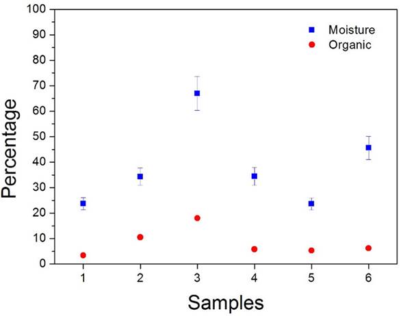
As mentioned in Sec. 2.2, the moisture and organic contents in both, analytical and reference sediment samples were removed by putting them through successive steps of drying and incineration. For a given mass of sample, the moisture and organic percentage contents were calculated from the weight reductions measured after the two steps, respectively. The results are exposed in Fig. 3, where the significant variations of the levels of moisture and organic contents of the samples coming from the different sites can be observed. After this process, any possible matrix effects, to which LIBS is particularly sensitive, were minimized.
3.2. Evaluation of LIBS analytical performance
Quantitative determination of the Cr and Cu contents in the sediment samples was accomplished with the calibration curve method. The line profiles of the Cr I and Cu I lines were recorded from the different reference samples. Calibration curves were constructed for Cr and Cu by plotting the measured net intensities versus the corresponding concentrations of the analytes (Fig. 4). The experimental errors corresponded to the standard deviations of the different measurements. In both cases, the experimental data showed linear trends for the measured concentration ranges, good sensitivities, and a negligible self-absorption. Moreover, the low dispersion of the data evidence that matrix effect was minimized.
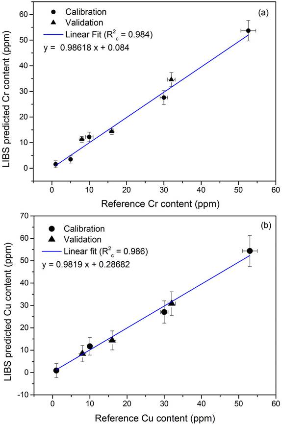
Figura 4 Correlation between concentration values determined by LIBS and the certified concentration values for (a) Cr and (b) Cu. The black circles are the calibration values and the black triangles are the values of validation samples.
To evaluate the analytical performance of the quantitative LIBS method, internal and external validation tests were accomplished. When self-absorption of the measured analytical lines and matrix effects in the samples are negligible a simple linear relationship between concentrations predicted by LIBS and the corresponding nominal values can be adopted. Hence, a model of linear correlation was used for Cr and Cu. The goodness of the model was determined by internal cross-validation with the calibrating samples in order to estimate the predictive power of the constructed calibration curves [41,42]. The external validation was performed with a set of 3 samples manufactured ad-hoc with Cr and Cu concentrations within the analyzed range to evaluate the robustness of the calibration curves. For both elements, the LIBS performance was evaluated through the correlation coefficient of cross-validation (R2cv) and the coefficient of calibration (R2c), together with the root-mean-square errors for prediction (RMSEP) and for calibration (RMSEC), respectively. Then, the relative standard errors; i.e. RSEC; RSEP) were calculated to account for the total errors (i.e. calibration and prediction) which allowed to evaluate the overall precision of the quantitative predictions [43].
The linear correlations from the univariate analysis carried out between the LIBS results for Cr and Cu concentrations and the corresponding nominal values are shown in Fig. 3. The results are presented in Table II. In both cases, the linear model yielded satisfactory results with correlation coefficients
Table II Cr and Cu regression performance evaluated by cross-validation (leave-one-out) and external validation (using the validation data set).
| Element | Calibration | Validation | |||||
|---|---|---|---|---|---|---|---|
|
|
RMSEC a |
|
RMSECV a | RSEC b | RMSEP a | RSEP b | |
| Cr | 0.978 | 1.71 | 0.985 | 2.96 | 6.20 | 2.59 | 12.26 |
| Cu | 0.986 | 1.83 | 0.981 | 3.58 | 5.94 | 1.18 | 5.61 |
a Expressed in ppm.
b Expressed in %.
3.3. Quantitative analysis
The calibration curves obtained for Cr and Cu are shown in Fig. 5. The data were fitted to straight lines. The experimental errors corresponded to the standard deviations of the measurements. It is observed that the linear regressions had non-zero intercepts that indicated initial concentrations for Cr: (46 ± 3) ppm, and Cu: (34 ± 4) ppm in the sediments sampled at point #3. These values were added to the concentrations of the reference samples in Fig. 5. These may be attributed to the natural quantities of the metals in the sediments [44,45]. Nevertheless, further measurements are required for a more accurate determination.
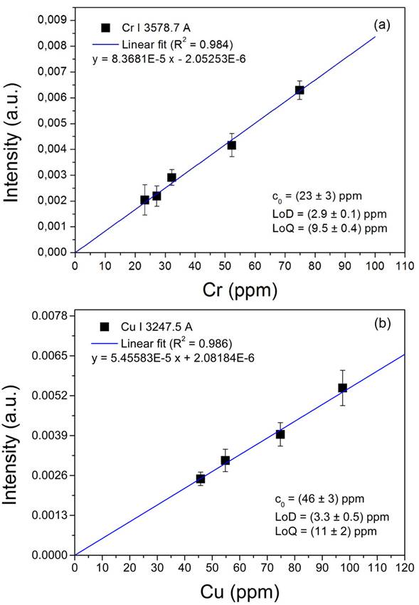
Figura 5 Calibration curves for (a) Cr and (b) Cu, constructed by the standard addition method. The natural concentrations (c 0) calculated in the reference samples, as well as the limits of detection (LoD) and quantification (LoQ) are indicated.
The limits of detection and quantification for Cr and Cu were evaluated for the present experimental conditions. The limit of detection (LoD) is defined as the minimum detectable concentration in the sample and it can be calculated as LoD = 3(σ/s), where σ is the standard deviation of the background, and s is the sensitivity of the analytical line given by the slope of the corresponding calibration curve [46]. The obtained limits of detection were 2.9 ppm for Cr, and 3.3 ppm for Cu. The limit of quantification (LoQ) is defined as the lowest concentration in the sample for an accurate quantification and it can be calculated as LoQ = 3:3 × LoD46. The obtained values were 9.5 ppm for Cr, and 11 ppm for Cu.
The Cr and Cu concentrations (ppm) in the analyzed sediments were determined by interpolating their measured net intensities of emission in the linear fitting functions. The obtained results are summarized in Table III. The errors were estimated from error propagation for the measured quantities.
Table III Cr and Cu concentrations for the sediments analyzed and baseline values.
| Samples | Cr (ppm) | Cu (ppm) | |
| 1 | 19±3 | 45±7 | |
| 2 | 25±3 | 42±7 | |
| 3 | 23±3 | 34±3 | |
| 4 | 24±4 | 27±1 | |
| 5 | 49±3 | 81±3 | |
| 6 | 33±6 | 59±11 | |
| CEQG a | TELb | 37.3 | 35.7 |
| PELc | 90 | 197 |
a Canadian Environmental Quality Guidelines (2003) [26].
b Threshold Effect Level.
c Probable Effect Level.
3.4. Evaluation of Langueyú stream pollution
In Fig. 6, the Cr and Cu concentrations obtained for the sediments at the different sampling points are compared with baseline values. Both, Cr and Cu concentrations showed marked increasing trends from upstream to downstream that can be linked to the influence of anthropogenic activities. Since in Argentina does not exist any regulation about toxic metals in sediments, the Canadian Environmental Quality Guidelines were used to assess the potential ecological risks of the heavy metals analyzed [47]. The Threshold Effect Level (TEL) is defined as the concentration value below which adverse biological effects are expected to occur rarely The Probable Effect Level (PEL) is defined as the value above which adverse effects are expected to occur frequently.
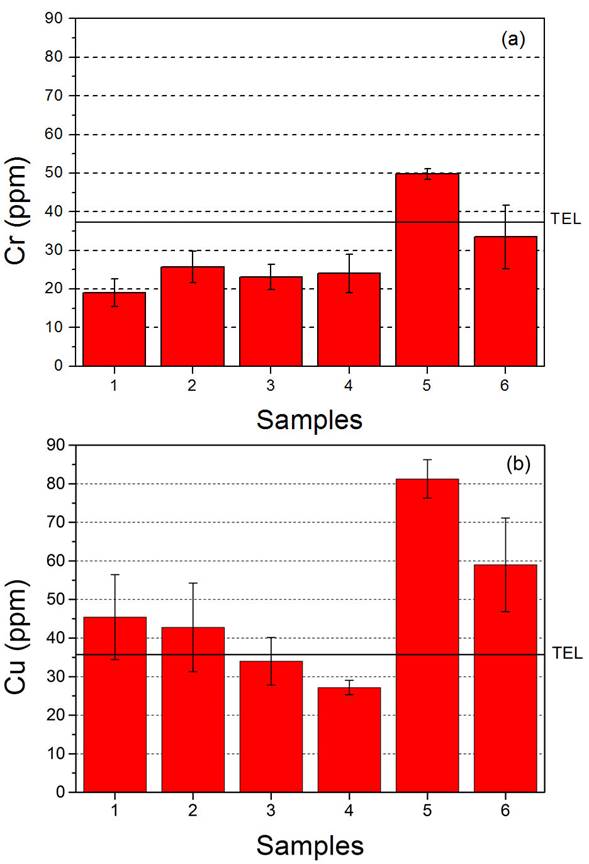
Figura 6 Cr (a) and Cu (b) concentrations in sediment samples. The baseline levels (TEL) are indicated.
All the measured Cr and Cu concentrations measured were below the PEL values. In turn, upstream (points #1-4), the Cr concentrations were clearly below the TEL value, and Cu concentrations were of the same order of the baseline value, within the experimental error. On the other hand, significant growths were observed downstream for Cr and Cu. The highest metal concentrations were measured at point #5 (Cr: 49 ppm and Cu: 81 ppm). Then, at point #6, the Cr concentration fell below the TEL value while the Cu concentration showed a slight decrease but remained well above the TEL value. These concentration increments evidence a sure pollution of the basin due to the nearby facilities which presumably discharge wastewater to the Langueyú stream with-out a proper treatment. Subsequently, the heavy metals in water precipitated into the sediments. The high Cr content can be associated to a tannery located at approximately 50 m from point #5, which used this metal during its production process. Despite the tannery was closed a few years ago, the Crenriched sediments indicated that its harmful effects persisted in the basin. The high Cu content may be associated to untreated effluents of industrial and/or domestic wastewater.
A contamination factor (CF) was calculated, defined as the ratio of heavy metal concentration measured in a given sediment over a reference concentration of the same element in a non-polluted area [48]. Namely, CF = CS=C RefS where C s is the total concentration in sediment and C RefS is the uncontaminated reference concentration in sediment; i.e. sample #3 in this study. According to this contamination factor, the contamination level may be classified as low degree (CF < 1), moderate degree (1 ≤ CF < 3), considerable degree (3 ≤ CF < 6), and very high degree (CF ≥ 6). The calculated CF values are exposed in Fig. 7, where it is observed that the sampling points #5 and #6 present a moderate contamination by Cr and Cu.
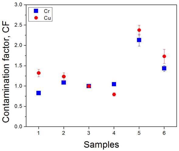
Because of the optically-thin emission of the plasmas generated as well as the negligible matrix effect in our experimental conditions, the total intensity ratios of the analytical lines are proportional to their concentrations in the samples. Therefore, the total intensities of emission of the heavy metals can be measured at the sampling point #5 to assess very fast the level of pollution of the stream and, then, evaluate if a more detailed sampling and analysis can be useful.
4. Conclusions
LIBS technique was applied for quantitative elemental analysis of Cr and Cu in fluvial sediments collected from Langueyú stream basin (Tandil, Argentina). The samples were prepared in pellets and analyzed with the standard addition calibration approach in which the moisture and organic matter contents of the sediments were taken into account to overcome the strong matrix effect. The analytical performance of the LIBS calibration method was evaluated by internal and external validation with very good statistical results. The limits of detection were 2.9 ppm for Cr and 3.3 ppm for Cu. The limits of quantification were 9.5 ppm for Cr and 11 ppm for Cu.
The obtained results showed that the concentrations of both, Cr and Cu were significantly increased downstream respect to the values measured upstream, with relative increments of about 53 % and 58 %, respectively. The level of contamination can be classified as moderate and constitutes a risk for human health and the environment. The increments of heavy metal concentrations can be linked directly to anthropogenic activities carried out by several industries that discharge their liquid effluents in the stream, as well as to the spills of a sewage treatment plant.
In addition, the optimization of LIBS analysis for the rapid reliable screening of heavy metal concentrations in sediment samples was demonstrated. It should be mentioned that LIBS technique is not competitive but complementary to other analytical techniques. In fact, it allows a monitoring and pre-selection of samples and analytes of interest which, if necessary, would be later examined with a more accurate analytical technique.

