


 text new page (beta)
 English (pdf)
 Article in xml format
 Article references
 Send this article by e-mail
 Cited by SciELO
  Similars in
SciELO
Similars in
SciELO 
 Permalink
1. Introduction
The compact objects: neutron stars, pulsars, strange stars have been approached from different perspectives, mainly through particle physics and gravitation, which have allowed us to describe their behavior at the microscopic and macroscopic levels respectively [1,2]. A consequence of the investigations carried out since the last century leads us to the fact that compact stars are constituted by electrons, neutrons and possibly quarks and that their equilibrium is in part due to the degeneration pressure among the particles. In the case of white dwarf stars this pressure of degeneration is due to the electrons and this consideration led to determine the so-called Chandrasekhar limit for the mass of this type of stars that corresponds to 1.44 solar masses [3,4], while the degenerating pressure of the neutrons implies that the mass of the neutron stars is approximately Mʘ. Stellar objects even more dense than these are constituted by quarks, although in reality these stars are hybrid, constituted predominantly by some of these particles. In the astrophysical aspect when we consider the microscopic behavior, particle interaction, we can introduce some equation of state associated to MIT bag model for the quark matter P = (1/3)(c2ρ - Bg) [5] or a polytropic state equation P = μρ1+1/n [6] if we refer to a neutron star or a white dwarf. Of course, there is a possibility that the interior of a star is decried by some other state equation P = P(ρ) depending on density orders [7-9] even if the state equation is not expressed implicitly, that is, F(P, ρ, S) = 0, where S represents some parameters or, in the case of electrically charged objects, include an electric charge relation. This may be the approach, although it is not indicated, present in some research reports in which solutions are found to Einstein’s equations with some source of matter that allows modeling compact stellar objects. Sometimes it is possible to determine a state equation, in the static and spherically symmetric case, since the pressure P = P(r) and density ρ = ρ(r) could get to express one in function of the other P = P(ρ) = 0 by inversion of the radial coordinate [10], although in general this does not happen due to the complexity of the solution.
However, the construction of stellar models, although it does not allow us to obtain any equation of state, guides us in a better understanding of the inner behavior of the stars through the use of gravitational theories such as the theory of Einstein’s General Relativity. For this theory, the vast majority of models or analyzes proposed near the interior of the star consider that it is described by a perfect fluid [11,12], a perfect fluid charged [13,14], an anisotropic fluid [13,14] or a charged anisotropic charged perfect fluid [13,18]. The class of solutions presented in each case attends to the type of objects that one wishes to describe or understand. The perfect fluid models are used for less compact stars, while the anisotropic or charged models allow to represent more compact stellar objects. Regarding the last case, there is a minimum value [19] for the ratio of mass and radius which generalizes to Buchdal [20]. Through a graphical analysis it has been shown that the compactness is even greater than the upper limit for a perfect fluid [21]. In this work we present a charged perfect fluid interior solution in the context of the Einstein- Maxwell theory, which is physically acceptable, i.e., satisfied with this feature.
The construction of a static and symmetrically spherical space-time is proposed from the assumption of a specific form of gravitational potential gtt [22] and the magnitude of the electric field. The solution satisfies conditions that make it physically acceptable and allows this to represent astrophysical compact stars with a compactness u ≤ 0.53379772212. In the Sec. sec2 we present the Einstein - Maxwell field equations for a charged perfect fluid charged fluid and the conditions are given for the solution to be physically acceptable. In the Sec. sec3 the solution of the field equations is presented and the validation intervals of the parameters are determined considering the physical conditions that must be satisfied, while in the Sec. 4 we determine the type of astrophysical objects that can be modeled and shown by graphical representations of the internal behavior, as well as an analysis of the possible values of density and pressure inside according to a stellar object with a solar mass. We finished the research work by presenting some conclusions in Sec. 5.
2. The system
Einstein-Maxwell field equations of gravitation for a perfect fluid charged are given
for
with P representing the pressure distribution, ρ the density distribution measured by an observer with velocity vector uμ, Fμν the Maxwell tensor and k = 8πG / c4. We consider the static and spherically symmetric metric of the interior in Schwartzschild coordinates [24]
We consider that the contribution of the Maxwell tensor is due to an electric field, so the non-zero components of the electric part are:
where
with q(r)the total charged inside a sphere of radius r. The field equations are write as [25]:
where ' denotes the derivative with respect to the coordinate r. This is the system of equations that we must solve for the construction of a stellar model given by a perfect charged fluid. The system has three Eqs. (4)-(6) for five functions (ρ, P, E, y, B) so two restrictions are required, in our case these are the shape of the gravitational potentiall gtt = -y2 and the function of the magnitude of the field E2, the choice of the first of these functions is motivated by previous work in which a perfect fluid neutral model has been developed, while the magnitude of the electric field is proposed so that we can represent objects with greater compactness than in the neutral case and with greater diversity of behavior. The solution to the Eqs. (4)-(6) requires to satisfy conditions that make it physically acceptable, which will be described in the next section.
2.1. Physicals conditions
For an inner solution of the Einstein-Maxwell equations with perfect fluid associated with compact objects to describe a physically acceptable model, the following conditions must be fulfilled [12]:
The solution must not have singularities, geometric or physical variables, i.e., for 0 ≤ r ≤ R the curvature scalars must be regular and the metric functions (y2, B), the density and pressure must be bounded.
The pressure and density must be positive and monotonically decreasing functions as a function of radial distance, with its maximum value in the center, in, particular in the origin:
while for r ≠ 0 ρ' < 0 and P' < 0.
The energy conditions must be [26]
NEC null energy condition ρ + P ≥ 0
WEC weak energy condition ρ ≥ 0 and ρ + P ≥ 0
SEC strong energy condition ρ + 3P ≥ 0 and ρ + P ≥ 0
DEC dominant energy condition ρ ≥ 0 and ρ ± P ≥ 0
From the previous requirement for density and pressure we have that the only additional restriction corresponds to the DEC.
The causation condition must not be violated, i.e. the magnitude of the speed of sound must be less than the speed of light
and additionally we will impose that the speed of sound is a monotonous function decreasing towards the surface.
There must be a region r = R, the surface of the star, where the pressure is zero P(R) = 0.
On the boundary r = R the interior solution should match continuously with an exterior Reissner-Nordstrom solution
This requires the continuity of y2(r), B(r) and q(r) = Q across the region r = R, where M and Q represent the total mass and charge inside the fluid sphere respectively.
Electric field intensity E is such that E(0) = 0 and taken to be monotonically increasing, i.e., dE / dr > 0 for 0 < r ≤.
These basic requirements allow to determine which interior solution can be useful as a model for the description of some compact object. As a result of the conditions mentioned above it is known that one characteristic of these models is that the radio mass ratio, as a generalization to the limit of Buchdahl [20] GM / c 2 R ≤ 4/9, has a maximum value
this expression implies the possibility of having solutions with a greater compactness value than 1/2 due to the effect of the charge Q, property that is relevant to our model. In addition to this inequality there is also a lower bound for the radio mass ratio
both relations have a good limit for the neutral case Q = 0.
Another important quantity in the stellar models that is associated with the mass
and the radius is the gravitational redshift on the surface
3. The solution and their analysis
The system of equations described in the previous section supports a solution with
in the case that the perfect fluid is neutral. In most previous investigations the
form of this function has been proposed as
and
So other functions can be proposed with these properties. The proposed form for the function y(r) and other similar functions have allowed to show the relevance of the existence of anisotropic pressures to be able to have physically acceptable models [31] besides that they have been applied for the description of physically acceptable stellar models [30,32,33], some of which are characterized because the speed of sound is a decreasing monotonic function as a function of the radial coordinate [34].
The construction of interior solutions is useful to have a better clarity of the inner behavior of the stars [12], some solutions with perfect fluid sources without charge [29,35,36] these became generalized to charged case [37-39] to represent compact stars.
The proposal of this section is to obtain a charged model that generalizes to the previously constructed case [22]. Some of the advantages presented by charged models is that their compactness ratio becomes greater than their counterpart without charge as a result of the non-neutrality of the fluid. The behavior of the electric charge or equivalently of the electric field E = q(r)/r2 as already mentioned in the previous section, it must be zero in the center and it must be a growing monotonous function, so in our case we choose the electric field in the form
v ≥ 0represents the charge parameter that in the case v = 0 will allow us to recover the solution without electric charge [22]. The shape of the electric field magnitude is not unique, there are a variety of possible acceptable functions for the same function y(r) [37-39], the choice of this serves particular interests of the approach of the model to be proposed or of the research proposed, even this can be given through the charge density [40] or through a relationship with the state equation [41].
In our case this form of the electric field was chosen so that the class of objects that can be represented can have a greater compactness, and this will be shown in the next section. Replacing this form of electric field and potential y in the Eqs. (5) y (6), after subtracting them, we come to the differential equation:
here we have defined H0(r) = 1 + 16ar2 - 30a2r4. The solution to this equation implies:
Where C is the constant of integration and
This determines the solution, i.e., the geometry and the hydrostatic functions, so that when replacing (9), (10) y (11) in the Eqs. (4) and (5) we obtain
where in the expression of density, Eq. (12), S1 = 150a2r4 + 1330a3r6 +10a4r8. Given the conditions that must be satisfied the solution to be physically acceptable, it is necessary to determine the speed of sound
due to its extension it is not written in the text, although it will be considered in the analysis of the conditions. The metric functions as well as the density, pressing and electric field are regular in the center, however, the explicit form of these is required in order to obtain the intervals of the system constants (a, C, v) as a result of the physical conditions described in the previous section. Then, from equations (12) and (13) as well as how the speed of sound is, we have:
According to the required conditions, each of these relationships must be positive, in addition to the speed of sound that must be smaller than the speed of light. On the other hand as ρ'(0) = 0, P'(0) = 0, density and pressure are decreasing monotone functions with their maximum in the center, so it is required that their second derivatives
be negative, while the electric field satisfies E(0) = 0, E'(0) = 0 y E2''(0) = 27va2; then v ≤ 0 as had been assumed in the Eq. (10). To the set of inequalities generated from the conditions required in the center for the solution to be physically acceptable expressed by (14)-(18), it is convenient to complement them with the relation obtained from the existence of the surface of the star, identified by P(R) = 0. Considering (13) in r = R we can get the constant C:
where w = aR2 with S2(w) = 200(1+65w+10w2)(1+w)6 and S3(w) = 2+179w+1902w 2+170w3+200w4. The set of inequalities is expressed only in terms of the dimensionless parameters (v,w). However, these conditions are only the content of the behavior in the object center. The parameter w is restricted by the condition that the electric field must be a growing monotonous function for all r ∈ [0,R]. This happens if inside the electric field has no maximum and the limit case occurs when at the border the electric field has a maximum, this is E2(R)' = 0 which implies that
since w > 0 then w is constrained by the smallest positive root of this equation, which is w = 0.13828732, this value of w is greater than the maximum value allowed when you have the perfect fluid without load whose value is w(q=0) = 0.1073273425. The maximum value of the parameter v it is determined by the condition that the speed of sound must be positive. The behavior of this function, for the solution we are analyzing, requires that the speed of sound at the border be positive and this happens if v ≤ vmax where
and S4 = 129600w468420w5 + 16200w6 + 1000w7. So the maximum value of v depends on w. The minimum value of v also depends on the specific value of w and is determined by the condition that the speed of sound is smaller than the speed of light, the value of r where this happens changes depending on the value of w. In particular for the maximum value of w = 0.13828732 the speed of sound matches the speed of light for v = 0.274043033 in r = 0.572156468R, so the range of v ∈ (0.27404 3033. 2.84837494). In general, the interval for v ∈ (vmin; vmax) and the value of vmin are not being determined so that the speed of sound is smaller than the speed of light.
4. Graphic analysis
The continuity of the metric and electric field allows us to determine the relationship which determines the compaction of the stellar objects that can be represented with the solution construed. The external geometry is given by the Reisner-Nordstrom solution
where M and Q are the mass and the electric charge of the star respectively. Evaluating the interior metrics in r = R and matching terms we get the reason for compactness
The value of compactness u = u(w,v) is a monotonically increasing function of both variables so the maximum value of compactness occurs for the maximum value of v and w. Evaluating this relation for the maximum value of v = vmax we obtain
where S5 = 7100w5 +
1000w6, while evaluating this expression for the
maximum permitted value of w w = 0.13828732 we obtain that the
maximum value of possible compactness is
umax = 0.5337972212, which compared
to the neutral case that has a compactness value of u =
0.3581350065, the effect of charge allows the representation of more compact objects
compared to the case without charge. Models not electrically charged allow a
compactness value accepted by the limit of Buchdahl, however for the charged case
the radius of the star could be smaller than the radius of Schwarzschild
u > 1/2 as it happens in our model, the reason is associated
with the effect of the charge. In the neutral case u = 1/2
indicates that the radius of the star coincides with the radius of Schwarzschild
rs = 2GM /
c2 which would imply the existence of a black hole.
However when the Einstein-Maxwell equations are considered in a static space-time,
spherically symmetric and asymmetrically flat, the respective black hole is given by
the geometry of Reissner - Nordstrom represented by the metric (7) and in this case the external event
horizon
Table I Values of the compactness for different values of the charged parameter with w = 0:13828732.
| v | 2.8483749 | 2.204792 | 1.5612094 | 0.9176260 | 0.2740430 |
| u | 0.5337971 | 0.4960593 | 0.4583215 | 0.4205838 | 0.3828460 |
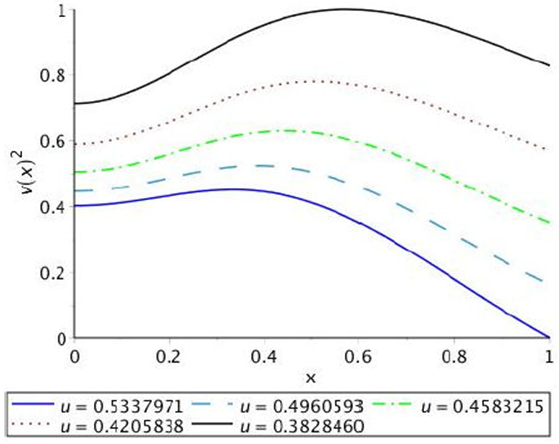
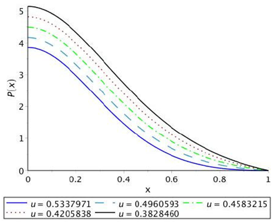
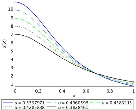
To graphically represent the behavior of density we define the dimensionless variable ρ → kc 2 R 2ρ as a function of x = r/R. On graph 2 its regular behavior is shown, bounded and monotone decreasing for different values of the parameter v with w = wmax. The central density is greater for the larger values of the charge parameter v while on the surface the opposite occurs. The graphic representation, Fig. 3, of the dimensionless function associated with pressure P → kR2P in terms of the function of x = r/R shows its monotonically decreasing behavior as well as bounded and positive. By the effect of the electric charge manifested through the parameter v the pressure associated with the perfect fluid is lower for higher values of this which allows denser objects. As can be seen from the comparison of Figs. 2 and 3 for greater compactness the density is greater and the pressure is lower. Figure 4 shows that the solution satisfies the condition required for the adiabatic index, γ > 4/3, which guarantees its stability.

From Fig. 5 an increase of the electric field strenght is observed as the electric charge increases.

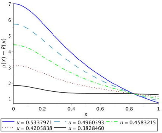
Another condition imposed for a model to be physically acceptable is that the energy conditions are satisfied since the density and the positive pressure are the same as the magnitude of the electric field E2. The only one that requires a verification is the dominate energy condition and this is shown graphically in the Fig. 6 where it is observed that this is satisfied.
The graphical representation of the hydrostatic functions presented in terms of dimensionless functions, is helpful to observe their behavior, however to obtain the ranges of the possible physical values of these functions, it is necessary to introduce the units to see that the values which the model are consistent with orders of magnitude associated with this type of objects. To determine the orders of magnitude of the density and the pressure below we consider a star with a mass equal to the mass of the sun and we obtain the values of the radius, pressure and central density as well as its density at the surface for the values of the compactness used for the graphics.
From the Table II, it is observed that the ranges of values of the central density ρc and the density on the surface ρb , are of the order of magnitude associated with compact stars. So also the central pressure Pc is consistent with the expected values. The values of the speed of sound in the center νc and on the surface νb are smaller than the speed of light, i.e., these do not violate the condition of causality and even in the case of greater compactness the speed of sound at the surface is zero. From the graphic behavior and the value of the adiabatic index γ in the center given in the table is obtained that the solution is stable, because γ > 4/3. Two other quantities given for the different values of compactness are the net charge and the value of gravitational redshift on the surface, both values are within the expected ranges [40].
Table II Values of the hydrostatic variables in the center and on the surface for different values of the compactness as well as M = Mʘ.
| u | 0.533797 | 0.496059 | 0.458322 | 0.420584 | 0.382846 |
| R(m) | 2765.976 | 2976.398 | 3221.473 | 3510.524 | 3856.563 |
| ρc (1019 Kg/m3) | 7.954465 | 5.769167 | 3.909380 | 1.658865 | 2.727820 |
| ρb (1018Kg/m3) | 5.369969 | 5.425123 | 5.303410 | 5.032169 | 4.638761 |
| Pc (1036P) | 2.421304 | 2.298425 | 2.080038 | 1.875830 | 1.667535 |
| v2c(c2) | 0.402442 | 0.447095 | 0.506627 | 0.589964 | 0.714951 |
| v2b (c2) | 0 | 0.163272 | 0.351349 | 0.570351 | 0.828586 |
| γ | 1.929431 | 1.443294 | 1.441248 | 1.498013 | 1.643794 |
| Q(1020C) | 1.648824 | 1.560997 | 1.421715 | 1.187770 | 0.713078 |
| zb | 1.257805 | 1.171623 | 1.094611 | 1.025251 | 0.962353 |
Finally we apply our model for the data of SAX J1808.4-3658 (SS1) star of mass M = 1.435 Mʘ and radio R = 707 km [42], its compactness value is u = 0.2996795, so the value of v is determined from the Eq. (22)
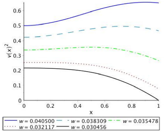
From the analysis of the restrictions for the model to be physically acceptable, we obtain that the validity interval of w ∈ [0.030456, 0.040500]. The only difference in the behavior of the functions for this data and the data for greater compactness is that there is now a subinterval of w ∈ [0.030456, 0.32117] in which the speed of sound is a decreasing monotone function. The Fig. 7 shows the behavior of the speed when there is no charge, w = 0.0405, being this a monotonously increasing function. In the charged case there are different behaviors for 0.032117 < w < 0.0405. The function of the speed of sound presents a region where it is monotonously increasing and another where it is growing monotonous. For w ∈ [0.030456, 0.032117] the speed of sound is monotonically decreasing as a result of the effect of the charge.
In the Table III, the values are shown with the magnitudes of the hydrostatic variables as well as the charge for the same parameter values w, in this it is observed that for the maximum value of the charge, the speed of sound on the surface approaches zero. In addition, the orders of magnitude of the densities are similar to the values reported with other models [40].
Table III Values of the hydrostatic variables in the center and on the surface SS1.
| w | 0.040500 | 0.038309 | 0.035478 | 0.032117 | 0.030456 |
| ν | 0 | 1.475197 | 3.952775 | 8.085688 | 10.79803 |
| Pc (1035P) | 2.207465 | 1.936262 | 1.526330 | 1.059583 | .8073013 |
| ρc (1018kg/m3) | 9.491643 | 7.652449 | 8.927432 | 8.523171 | 7.748338 |
| ρb (1018 kg/m3) | 2.908835 | 2.767600 | 2.572201 | 2.318696 | 2.183865 |
| vc (c2)2 | .5000328 | .4219832 | .3371526 | .2531569 | .2166285 |
| vb (c2)2 | 0.652298 | 0.465718 | 0.264912 | 0.076179 | 0.000004 |
| Q(1020C) | 0. | 1.223631 | 1.875167 | 2.459075 | 2.711817 |
| γ | 1.908003 | 2.109820 | 1.911706 | 2.236546 | 1.455289 |
5. Conclusions
Here we have obtained a charged perfect fluid solution that generalized a perfect fluid uncharged solution in a spacetime static and spherically symmetric. The solution depends of two parameters w and v the latter related to charge. The built solution considers a new form of gravitational potential gtt = (1+10ar3)3/(1+ar2)3 [22] and a particular form of the increasing monotonous charge, this is the one that generates different profiles of behavior of the speed of sound, differing from the case without charge where the speed is only monotone increasing. Another point in which the electric charge generates changes with respect to the case without electric charge is that the maximum umax = 0.5337972212 is much higher than at the maximum possible value for a perfect neutral fluid u < 4/9.
This remarkable characteristics of the model, as far as we know, have not been reported previously analytic solutions with such large compactness values, although in previous reports mention has been made of the possibility of having electrically charged models with greater compactness than 4/9, upper bound for the case of a perfect fluid neutral [21].
As a result of the analysis of the solution we have that the density and pressure, as radial functions, are monotonous, decrescent, bounded and regular. Additionally, considering the data of a star with mass Mʘ, we have it has that the orders of magnitude that the model generates with respect to density and pressure are consistent with those expected for neutron stars or quarks, with the advantage of having a range of possible values of the density, which, as expected, stars with the same radius and mass data may have different internal behavior. In our case what determines in a specific way the internal structure of the stars is the charge. On the other hand, the adiabatic index is a growing monotonous function and γ > 4/3 which guarantees stability. We also show that the model for smaller values of compactness, in particular for u = 0.2996795 can be associated with the data of the star J1808.4-3658(SS1). There is a parameter range w in which the speed of sound is a decreasing monotonous function, characteristic that some authors consider as desirable for some models.
Finally, it is worth mentioning that although the graphical analysis and physical hydrostatic values were presented for specific parameters, the behavior for other values of the parameters, is similar so it is concluded that the model can be used for other compact stars u < 0.5337972212. This work gives rise to some questions that could be developed in the future, such as what are the characteristics that the electric field function must have that allows to represent compact objects with a wide spectrum of possibilities in the representation of highly compact objects. Another question is the construction and analysis of an anisotropic charged model which generalizes the one presented here and the determination of the effect of the anisotropy and the electric charge and their comparison between both of them.

