


 text new page (beta)
 English (pdf)
 Article in xml format
 Article references
 Send this article by e-mail
 Cited by SciELO
  Similars in
SciELO
Similars in
SciELO 
 Permalink
1. Introduction
The Non Relativistic Schrödinger equation (SE) is one of the central equations in quantum physics which still attracts strong interest of both physicists and mathematicians. However, solving this equation is often very difficult, also obtaining exact analytic solutions may be found only for few cases [1]. Many advanced mathematical methods have been used to solve it. Among the most popular methods are Nikiforov-Uvarov method (NU) [2-10], asymptotic iteration method (AIM) [11-16], supersymmetric shape invariance approach (SUSY QM) [17-22], factorization method [23], exact/proper quantization rule [24-26], 1/N shifted expansion method [27] and Modified Factorisation Method [28-29] which could help to obtain approximate solutions of these wave equations in the presence of a suitable approximation scheme.
Hulthen potential is one of the crucial molecular potentials used in different areas of Physics such as nuclear and particle, atomic and condensed matter Physics and chemical Physics to describe the interaction between two atoms [30]. The q deformed Hulthen potential is of the form [35]
[29] noted that there are no differences between the behavior of the modified Yukawa potential and the inversely quadratic Yukawa potential [31] or the Yukawa potential [32]. Its application to diverse areas of physics has been of great interest and concern in recent times [33,34].
The generalized inverse quadratic Yukawa potential (GIQYP) is a superposition of the inverse quadratic Yukawa (IQY) and the Yukawa potential. It is asymptotic to a finite value as r → ∞ and becomes infinite at r = 0 [36]. The Generalized inverse quadratic Yukawa potential model is of the form [36]
The Generalized inverse quadratic Yukawa potential reduces to a constant potential when A = B = 0.
The study of dimensions plays an important role in many areas of physics and the extension of physical problems to higher dimensional space is of great interest. [37] noted that the exact solutions of both the relativistic and nonrelativistic wave equation with certain physical potential in higher dimensions are remarkably important not only in physics and chemistry, but also in pure and applied mathematics.
Recently, there has been great interest in combining of two or more potentials in
both the relativistic and non-relativistic regime. The essence of combining two or
more physical potential models is to have a wider range of applications [38]. For example, Hellmann [39], studied Schrödinger equation
with a superposition of Coulomb potential and Yukawa potential, this potential is
named Hellmann potential. His result is applicable in the area where both Coulomb
potential and Yukawa potential respectively find applications. Bearing this in mind,
we attempt to study the D-dimensional Schrödinger equation with a newly proposed
potential obtained from a combination of
where V1 is the coupling strength of the potential, α is the screening parameter and V0 is strength of the potential.
The organization of the work is as follows: In the next section, review the Nikiforov-Uvarov method. In Sec. 3, this method is applied to obtain the bound state solutions. In Sec. 4, we obtain numerical results while in Sec. 5 we discuss some special cases and in Sec. 6, we give the concluding remark.
2. Review of Nikiforov-Uvarov method
The Nikiforov-Uvarov (NU) method is based on solving the hypergeometric-type second-order differential equations by means of the special orthogonal functions [2]. The main equation which is closely associated with the method is given in the following form [40-41]
Where σ(s) and
σ(s) are polynomials at most second-degree,
The exact solution of Eq. (2) can be obtained by using the transformation
This transformation reduces Eq. (2) into a hypergeomet- ric-type equation of the form
The function Φ(s) can be defined as the logarithm derivative
where
With π(s) being at most a first-degree polynomial. The second ψ(s), being yn (n) in Eq. (3), is the hypergeometric function with its polynomial solution given by Rodrigues relation
Here, Bn is the normalization constant and ρ(s) is the weight function which must satisfy the condition
It should be noted that the derivative of τ(s) with respect to s must be negative. The eigenfunctions and eigenvalues can be obtained using the definition of the following function π(s) and parameter λ, respectively:
where
The value of k can be obtained by setting the discriminant of the square root in Eq. (9) equal to zero. As such, the new eigenvalue equation can be given as
3. Bound state solution with q deformed Hulthen and generalized inverse quadratic Yukawa potential in D dimension
The radial Schrödinger equation in D dimension can be written as [42]:
where μ is the reduced mass, Enl is the energy spectrum, ħ is the reduced Planck’s constant and n and l are the radial and orbital angular momentum quantum numbers respectively (or vibration-rotation quantum number in quantum chemistry). Substituting Eq. (1) into Eq. (15) gives:
Simplifying further Eq. (16) becomes;
Employing the Pekeris type approximation scheme [43], which is given by
Eq. (18) becomes;
Eq. (19) can be simplified introducing the following dimensionless abbreviations
And using the transformation s = e-2αr so as to enable us apply the NU method as a solution of the hypergeometric type
Comparing Eq. (19) and Eq. (2), we have the following parameters
Substituting these polynomials into Eq. (9), we get π(s) to be
where
To find the constant k the discriminant of the expression under the square root of Eq. (21) must be equal to zero. As such, we have that
Substituting Eq. (26) into Eq. (24) yields
From the knowledge of NU method, we choose the expression π(s) whose function τ(s) has a negative derivative. This is given by
with τ(s) being obtained as
Referring to Eq. (10), we define the constant λ as
Substituting Eq. (27) into Eq. (11) and carrying out simple algebra, where
and
we have
Substituting Eqs. (17) into Eq. (30) yields the energy eigenvalue equation of the q-deformed Hulthen potential and Generalized Inverse Quadratic Yukawa Potential in D dimension in the form
The corresponding wave functions can be evaluated by substituting π(s) and σ(s) from Eq. (27) and Eq. (23) respectively into Eq. (7) and solving the first order differential equation. This gives
The weight function ρ(s) from Eq. (7) can be obtained as
From the Rodrigues relation of Eq. (6), we obtain
where
Substituting Φ(s) and yn (s) from Eq. (32) and Eq. (34) respectively into Eq. (3), we obtain
4. Deductions from Eq. (34)
In this section, we take some adjustments of constants in Eq. (1) and (2) to have the following cases:
Coulomb plus inverse-square potential
If we set C = 0, α → 0, q = 1 Eq. (3) reduces to the Coulomb plus Inverse-Square Potential [44,58]:
Eq. (36) is also known as the Kratzer-Feus potential, this potential was studied by Ref. [58] in arbitrary dimensions. If we set ħ = µ = 1, Eq. (36) fully agrees with the result reported in Eq. (28) of Ref. [58]. Eq. (37) is also consistent with the result obtained in Eq. (15) of Ref [44].
Generalized inverse quadratic Yukawa potential
If V 0 = 0, q = 1 Eq. (3) reduces to the Generalized Inverse Quadratic Yukawa potential
and the energy Eq. (34) becomes
Equation (42) is the Energy Eigenvalue Equation for Generalised Inverse Quadratic Yukawa potential in D dimension. When D = 3, Eq. (42) is in full agreement with the results in Eq. (27) of Refs. [36].
Hulthen potential
If V1 = 0, and V0 = Ze2α Eq. (3) reduces to the q deformed Hulthen potential
and the energy equation Eq. (31) becomes
Equation (44) is the energy equation for the q deformed Hulthen potential in D Dimensions. If we set q = 1, α → α/2, it reduces to the energy equation for the Hulthen potential in D dimension
Equation (44) is identical with the energy eigenvalue equation given in Eq. (33) of Ref. [53]. Mores so, if we set D = 3, we arrive at the energy eigenvalue equation for the Hulthen potential in 3D.
Equation (46) is identical to the energy eigenvalues formula given in Eq. (34) of Ref. [53], Eq. (35) of Ref. [54], Eq. (27) of Ref. [55] and, Eq. (31) of Ref. [56] and Eq. (39) of Ref. [57].
Kratzer potential
If α → 0 and V0 = 0, q = 1 and setting A = -V1, B = 2V1 and C = -V1, Eq. (3) reduces to
Equation (31) becomes
Equation (48) is the Energy eigenvalue equation for the Kratzer potential in D dimensions. If D = 3 reduces to energy equation for Kratzer potential in 3D, which is very consistent with the result obtained in Eq. (28) of Ref. [45]
Inversely quadratic Yukawa potential
If V0 = 0, q = 0 and B = C = 0 the potential Eq. (3) reduces to the Inverse Quadratic Yukawa Potential [33]:
Eq. (34) becomes
Equation (50) is the energy equation for the Inverse Quadratic Yukawa Potential in D Dimensions. If D = 3, Eq. (50) reduces to the energy equation in 3D, which is identical to the results in Eq. (40) of Ref. [46], Eq. (21) of Ref. [45] and Eq. (50) of Ref. [47].
Yukawa potential
If V0 = 0, and A = C = 0 the potential Eq. (3) reduces to the Yukawa Potential
Equation (52) is the energy eigenvalue equation for the Yukawa potential in D dimensions. If D = 3, Eq. (52) becomes identical with Eqs. (50) and (17) reported in Ref. [48] and [49], respectively.
q Deformed Hulthen potential plus inversely quadratic Yukawa potential
If B = C = 0 the potential Eq. (3) reduces to the q Deformed Hulthen Potential plus Inversely Quadratic Yukawa Potential
Equation (51) is the energy equation for qDHPIQYP in D Dimensions. If D = 3, Eq. (51) reduces to the energy equation for qDHPIQYP in 3D. Hence, this is in agreement with the result reported in Eq. (21) of Ref. [50].
Wood saxon
If V1 =0, q → 0, the potential Eq. (3) reduces to the Wood-Saxon Potential [51]
Equation (56) is the energy equation for Woood saxon potential in D Dimensions. If D = 3, Eq. (56) reduces to energy equation for Wood Saxon potential in 3D which is in agreement with Eq. (33) of Ref. [51,52].
Coulomb potential
If V0 = 0, A = C = 0, α → 0the potential Eq. (3) reduces to the Coulomb Potential [53]
Equation (58) is the energy equation for Coulomb potential in D Dimensions. This result is consistent with the result obtained in Eq. (7.14) of Ref. [37]. Also, comparing our work with the result gotten in Eq. (32) of Ref. [38], it is worthy to note here that the authors in Ref. [38] failed to set the screening parameter (i.e. δ in Eq. (32) of Ref. [38]) equal to zero. If that is done, then there would be a clear consistency in the energy eigenvalue equation gotten in our Eq. (58) and Eq. (32) of Ref. [38]. More so, when D = 3, Eq. (58) reduces to the energy equation for Coulomb potential in 3D. This result is in agreement with the result obtained in Eq. (101) of Ref. [41].
5. Discussion
In Table I, we present the numerical results for q-deformed HPGIQYP in natural units for undisturbed system q = 1 and low potential strength, V0 = 0.05 eV and coupling strength eV. It is observed that the energy decreases as the orbital angular momentum increases for any given value of the principal quantum number n in all dimensions. Physically, a particle in this potential is highly bound and becomes more attractive as increases. Interestingly, the above observation is the same with and without the presence of the deformation parameter in the system as shown in Table II for which q =2.
Table I The bound state energy levels (in units of fm-1) of the q deformed HPGIQYP for various values of n, l and for ħ = μ = 1, V 1 = 0:05, V 0 = 0:06, α = 0:1 and q = 1.
| D | l | E0 | E1 | E2 | E3 | E4 | E5 |
| 1 | 0 | -0.111532657 | -0.050160469 | -0.061805001 | -0.091588170 | -0.133612341 | -0.186495563 |
| 1 | -0.111532657 | -0.050160469 | -0.061805001 | -0.091588170 | -0.133612341 | -0.186495563 | |
| 2 | -0.050001470 | -0.063637479 | -0.094491464 | -0.137403514 | -0.191119393 | -0.255212929 | |
| 3 | -0.063963864 | -0.095000000 | -0.138064566 | -0.191923889 | -0.256157355 | -0.330589834 | |
| 2 | 0 | - | - | - | - | - | - |
| 1 | -0.057730423 | -0.053663600 | -0.076861376 | -0.113796613 | -0.162002377 | -0.220756343 | |
| 2 | -0.054040856 | -0.077671011 | -0.114918947 | -0.163406670 | -0.222431895 | -0.291727413 | |
| 3 | -0.077934315 | -0.115282910 | -0.163861568 | -0.222974330 | -0.292355951 | -0.371887520 | |
| 3 | 0 | -0.111532657 | -0.050160469 | -0.061805001 | -0.091588170 | -0.133612341 | -0.186495563 |
| 1 | -0.050001470 | -0.063637479 | -0.094491464 | -0.137403514 | -0.191119393 | -0.255212929 | |
| 2 | -0.063963864 | -0.095000000 | -0.138064566 | -0.191923889 | -0.256157355 | -0.330589834 | |
| 3 | -0.095215754 | -0.138344769 | -0.192264742 | -0.256557384 | -0.331048371 | -0.415654558 | |
| 4 | 0 | -0.057730423 | -0.053663600 | -0.076861376 | -0.113796613 | -0.162002377 | -0.220756343 |
| 1 | -0.054040856 | -0.077671011 | -0.114918947 | -0.163406670 | -0.222431895 | -0.291727413 | |
| 2 | -0.077934315 | -0.115282910 | -0.163861568 | -0.222974330 | -0.292355951 | -0.371887520 | |
| 3 | -0.115463942 | -0.164087740 | -0.223243964 | -0.292668339 | -0.372242321 | -0.461906307 | |
| 5 | 0 | -0.050001470 | -0.063637479 | -0.094491464 | -0.137403514 | -0.191119393 | -0.255212929 |
| 1 | -0.063963864 | -0.095000000 | -0.138064566 | -0.191923889 | -0.256157355 | -0.330589834 | |
| 2 | -0.095215754 | -0.138344769 | -0.192264742 | -0.256557384 | -0.331048371 | -0.415654558 | |
| 3 | -0.138499958 | -0.192453483 | -0.256778864 | -0.331302223 | -0.415940595 | -0.510650327 |
Table II The bound state energy levels (in units of fm-1) of the q deformed HPGIQYP for various values of n, l and for ħ = μ = 1,
| D | l | E0 | E1 | E2 | E3 | E4 | E5 |
| 1 | 0 | -0.055540550 | -0.054743460 | -0.076688104 | -0.110461693 | -0.154758568 | -0.209260208 |
| 1 | -0.055540550 | -0.054743460 | -0.076688104 | -0.110461693 | -0.154758568 | -0.209260208 | |
| 2 | -0.050713075 | -0.067097009 | -0.096794134 | -0.137281881 | -0.188051277 | -0.248945654 | |
| 3 | -0.060304344 | -0.086357884 | -0.123577555 | -0.171174400 | -0.228929320 | -0.296761967 | |
| 2 | 0 | -0.062855099 | -0.052655813 | -0.072364751 | -0.104407142 | -0.147071045 | -0.199969056 |
| 1 | -0.050377886 | -0.059888551 | -0.085683732 | -0.122678251 | -0.170057863 | -0.227598190 | |
| 2 | -0.054379255 | -0.075979470 | -0.109478988 | -0.153516061 | -0.207762252 | -0.272106443 | |
| 3 | -0.068012053 | -0.098139551 | -0.139023045 | -0.190178724 | -0.251455966 | -0.322795574 | |
| 3 | 0 | -0.055540550 | -0.054743460 | -0.076688104 | -0.110461693 | -0.154758568 | -0.209260208 |
| 1 | -0.050713075 | -0.067097009 | -0.096794134 | -0.137281881 | -0.188051277 | -0.248945654 | |
| 2 | -0.060304344 | -0.086357884 | -0.123577555 | -0.171174400 | -0.228929320 | -0.296761967 | |
| 3 | -0.077274238 | -0.111271926 | -0.155781564 | -0.210492483 | -0.275298367 | -0.350154842 | |
| 4 | 0 | -0.050377886 | -0.059888551 | -0.085683732 | -0.122678251 | -0.170057863 | -0.227598190 |
| 1 | -0.054379255 | -0.075979470 | -0.109478988 | -0.153516061 | -0.207762252 | -0.272106443 | |
| 2 | -0.068012053 | -0.098139551 | -0.139023045 | -0.190178724 | -0.251455966 | -0.322795574 | |
| 3 | -0.087972214 | -0.125723307 | -0.173833646 | -0.232096027 | -0.300433652 | -0.378812734 | |
| 5 | 0 | -0.050713075 | -0.067097009 | -0.096794134 | -0.137281881 | -0.188051277 | -0.248945654 |
| 1 | -0.060304344 | -0.086357884 | -0.123577555 | -0.171174400 | -0.228929320 | -0.296761967 | |
| 2 | -0.077274238 | -0.111271926 | -0.155781564 | -0.210492483 | -0.275298367 | -0.350154842 | |
| 3 | -0.100039710 | -0.141473606 | -0.193167160 | -0.254977708 | -0.326848638 | -0.408753857 |
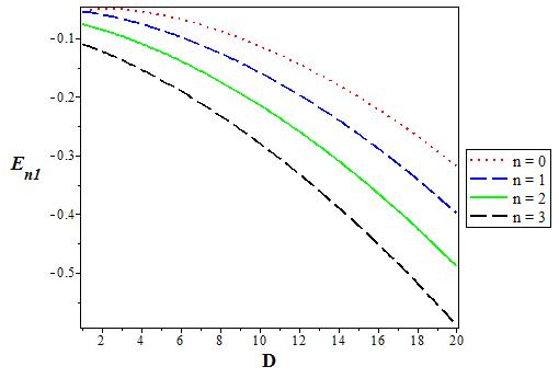
Figure 1-5 show the variations of potential versus r for different values of q, considering three potentials and four orbital angular momentums. In Figs. 6 and 7, we show the 3D variations of the energy with q for s-wave and p-state for different n. We repeat the same for the screening parameter α in Fig. 8 and 9. The energy increases when the potential strength V 0 increases, but behaves the other way roundfor coupling strength V1 as shown in Fig. 10-13. Finally, Figs. 14-17 shows the variation of energy level for various dimension D for the s-wave and p-state. The energy decreases when the dimension D increases in both cases and peaks at D = 2.
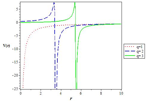
Figure 1 The variation of the q deformed Hulthen potential plus Generalized inverse quadratic Yukawa potential for various values of the deformation parameter (q+) as a function r. We choose V1 = 0:5, V0 = 0:6 and α = 0:1.
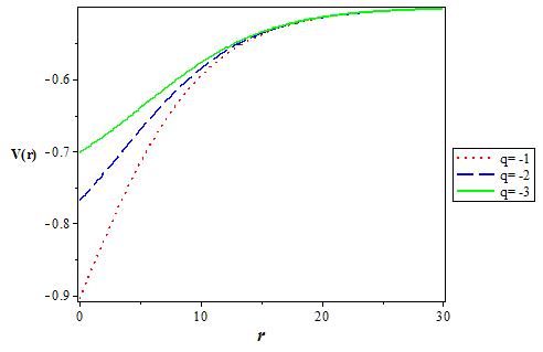
Figure 2 The variation of the q deformed Hulthen potential plus Generalized inverse quadratic Yukawa potential for various values of the deformation parameter (q-) as a function r. We choose V1 = 0:5, V0 = 0:6 and α = 0:1.
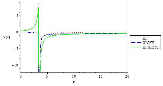
Figure 3 The variation of the q deformed Hulthen potential, Generalized inverse quadratic Yukawa potential and q deformed Hulthen potential plus Generalized inverse quadratic Yukawa potential as a function r. We choose V1 = 0:5, V0 = 0:6, q = 2 and α = 0:1.
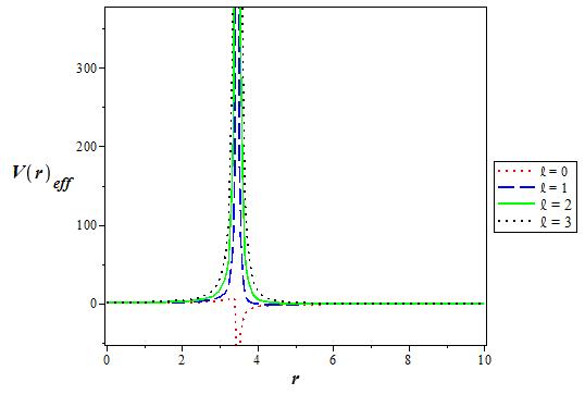
Figure 4 The variation of the effective q deformed Hulthen potential plus Generalized inverse quadratic Yukawa potential for various values of l as a function r. We choose V1 = 0:5, V0 = 0:6, q = 2 and α = 0:1 in 3D.
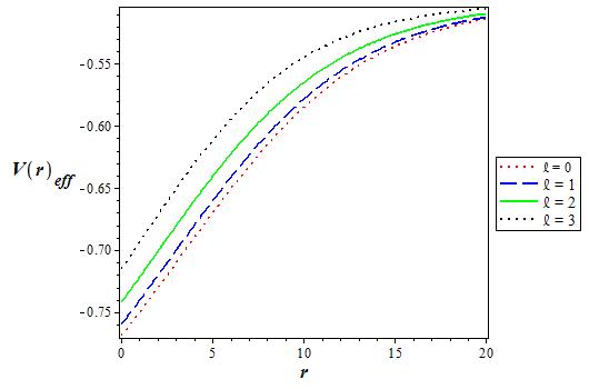
Figure 5 The variation of the effective q deformed Hulthen potential plus Generalized inverse quadratic Yukawa potential for various values of l as a function r. We choose V1 = 0:5, V0 = 0:6, q = -2 and α = 0:1 in 3D.
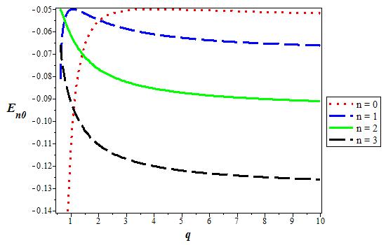
Figure 6 The variation of the s state (l = 0) energy level for various n as a function of the deformation parameter. We choose V1 = 0:05, V0 = 0:06, and α = 0:1 in 3D.
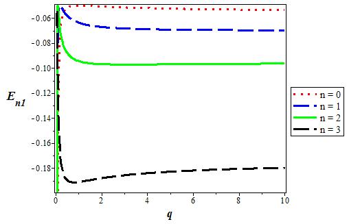
Figure 7 The variation of the p state (l = 1) energy level for various n as a function of the deformation parameter. We choose V1 = 0:05, V0 = 0:06, and α = 0:1 in 3D.
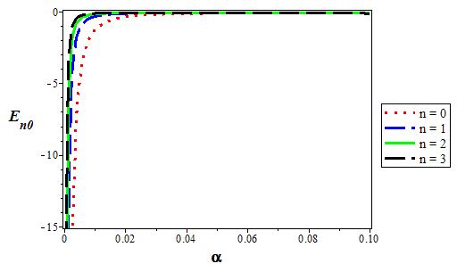
Figure 8 The variation of the s state (l = 0) energy level for various n as a function of the screening parameter (α). We choose V1 = 0:05, V0 = 0:06, and q = 2 in 3D.
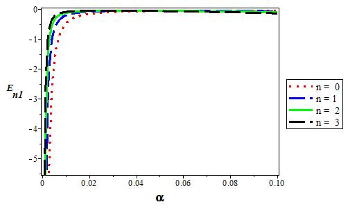
Figure 9 The variation of the p state (l = 1) energy level for various n as a function of the screening parameter (α). We choose V1 = 0:05, V0 = 0:06, and q = 2 in 3D.
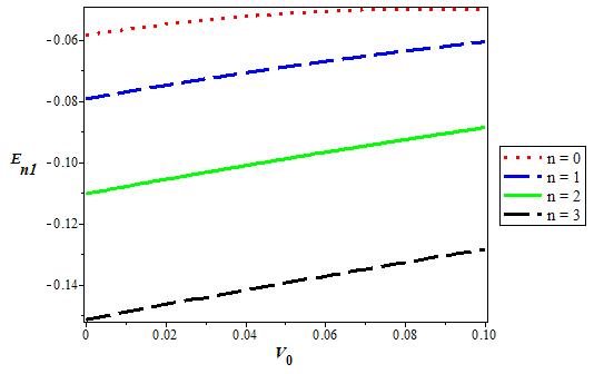
Figure 10 The variation of the p state (l = 1) energy level for various n as a function of the coupling strength V0. We choose V1 = 0:05, α = 0:1, and q = 2 in 3D.
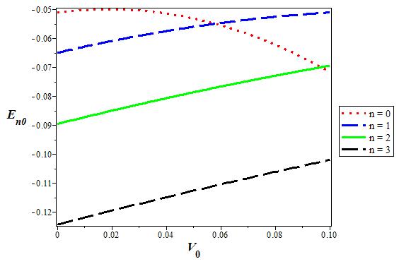
Figure 11 The variation of the s state (l = 0) energy level for various n as a function of the coupling strength V0. We choose V1 = 0:05, α = 0:1, and q = 2 in 3D.
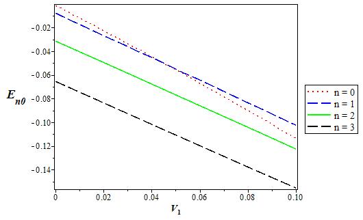
Figure 12 The variation of the s state (l = 0) energy level for various n as a function of the coupling strength V 1. We choose V0 = 0:06, α = 0:1, and q = 2 in 3D.
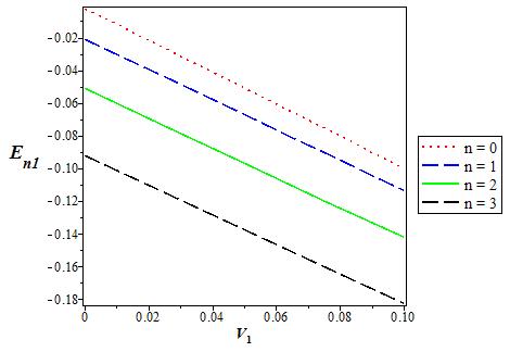
Figure 13 The variation of the p state (l = 1) energy level for various n as a function of the coupling strength V1. We choose V0 = 0:06, α = 0:1, and q = 2 in 3D.
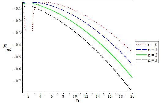
Figure 14 The variation of the p state (l = 0) energy level for various D as a function of the coupling strength V1. We chooseV0 = 0:06, V1 = 0:05, α = 0:1, and q = 1.
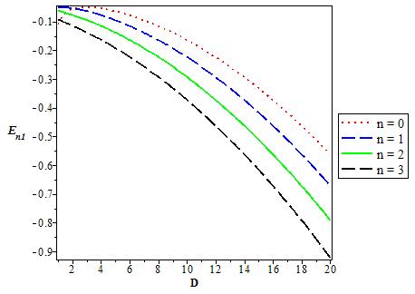
Figure 15 The variation of the p state (l = 1) energy level for various D as a function of the coupling strength V1. We choose V0 = 0:06, V1 = 0:05, α = 0:1, and q = 1.
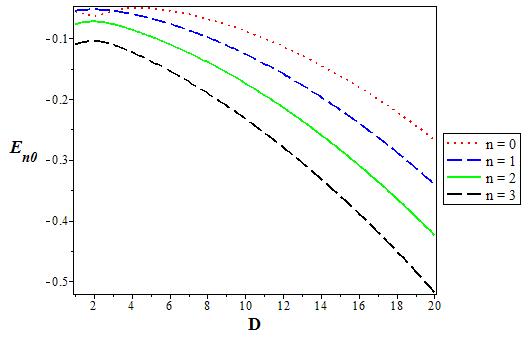
Figure 16 The variation of the s state (l = 0) energy level for various D as a function of the coupling strength V1. We choose V0 = 0:06, V1 = 0:05, α = 0:1, and q = 2.
6. Conclusion
In this work, we have studied the bound state solutions of the Schrodinger equation with q deformed Hulthen plus generalized inverse quadratic Yukawa potential using NU method. By making appropriate approximation to deal with the centrifugal term, we obtain the energy eigenvalues and the corresponding eigenfunctions and also discussed some special cases of the potential. We have calculated numerical energy eigenvalues and presented plots for various values of the potential parameters and found that the energy decreases as dimension increases. The results are in excellent agreement with literature.

