


 nueva página del texto (beta)
 Inglés (pdf)
 Artículo en XML
 Referencias del artículo
 Enviar artículo por email
 Citado por SciELO
  Similares en
SciELO
Similares en
SciELO 
 Permalink
1. Introduction
Polymers made of ionic fragments in their structure, which are considered by their iconicity level, or polymers composed entirely of ionic units are widely studied. Classical ionic polymers with sulfonate or carboxylate groups have been studied expansively but the diversity of anionic polymers is much more limited as compared with cationic polymers due to the fact that cationic polymers can be easily and more flexibly synthesized [1]. Most reported cationic polymers are based on amines or quaternary ammonium ions because of their basicity, relative stability, versatility and ease of access. Although of the number of polymer chemical structures has been multiplied, varying the physical properties, most of works have brought little innovation from the synthetic point of view [2,3]. One of the most studied properties for ionic polymers is the conductivity, which is not necessarily increased by increase the number of ionic centers in the corresponding ionic monomer. On the other hand, large ionic units with numerous ionic centers are not the best options for achieving high conductivity due to the electrostatic repulsion and steric impediments between bordering centers [4]; in contrast, ionic polymers with aprotic cations possess higher conductivity than their protic analogues [5].
There is a cycle of works related to the synthesis and characterization of polymers that contain vinylbenzyl trimethyl ammonium fragment in their structure and most of these works are aimed to the preparation of ionic membranes [6-11]. However, polymer preparation by polymerization of cationic monomers is based on known synthetic methods but determining the molecular weight by gel permeation chromatography (GPC) is a trial and error process. The GPC characterization of the resulting charged polymers requires a very specific combination of the mobile phase with salt but the charged polymers tend to adhere to certain columns. Some authors have reported difficulties in obtaining reliable molecular weights for charged copolymers because these measurements depend on the eluent type and solution’s pH, which are factors that make difficult the use of GPC for charged polymers [12-14]. When the ionic polymers contain groupers or blocks of polystyrene or some other fragments with low solubility in aqueous media such as BFˉ4, Tfˉ, and PF6ˉ (but not simple Brˉ) anions, the problem of molecular weight measurement for ionic polymers can be solved by using non-aqueous solvents such as Dimethylformamide (DMF), acetonitrile, etc. [12,14,15], or a combination of these with the aqueous solution of the salts 0.05M NaNO3, and 0.01M Na2HPO4 [13].
However, the measurement of molecular weights for water-soluble terpolymers with three different types of groupers and positive charge is not so trivial. Furthermore, the problem gets worse when the molecular weight of the terpolymer increases.
The development of interconnections between the measurement of molecular weights for water-soluble high molecular weight ionic polymers and molecular simulation is a pioneering field. Although ionic polymers and their synthesis methods are well known and new structures are in continuous development, their theoretical understanding is still an innovative area. The molecular weight dependence is revealed in the classical Fox-Flory equation [16-18], where the connection between total number density of polymers and the unperturbed radius of gyration of polymer is also given [19-24].
The procedure to estimate the molecular weight of ionic polymer is divided into four main parts. In the first section, the numerical model is presented and its results are shown and discussed in the second part. The third section is focused on describing the viscosity experimental data of the polymer in brine, their connection with the numerical model, and the prediction of the molecular weight. Finally, the conclusions are featured in the last section.
2. The model
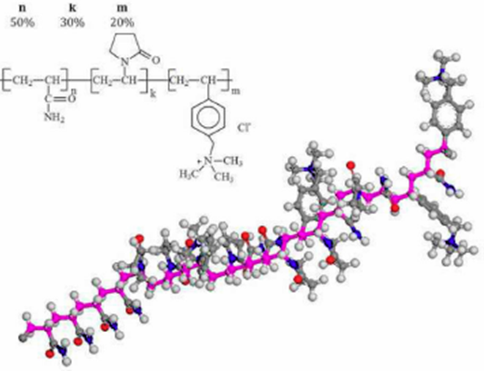
The structure of poly[acrylamide-co-vinylpyrrolidone-co-(vinylbenzyl) trimethylammo - nium]chloride is shown in Fig. 1. In the molecular structure, n, k, and m are the number of acrylamide, vinylpirrolidone, and (vinylbenzyl) trimethyl ammonium monomers, respectively. The monomer configurations are n/L =0.5, k/L = 0.3, and m/L = 0.2 where L = n+k+m is the total number of monomers. The polymer model was constructed by using the molecular editor of the Material Studio software. Its geometry and charge distribution were optimized by using the DMol3 module included in Material Studio. In another case, the procedure to construct the polymer molecule is also used to construct the water molecule.
The brine solution configuration with or without polymer are shown in Table I. In the cases of brine with polymer, the number of water molecules is calculated by assuming a polymer concentration of 1% of the total water weight. Clearly, the number of total molecules increases quickly with the number of polymers and hence, the cost of computational time becomes a problem. On the other hand, the proposed molecular system does not take into account the polymer-polymer interactions and this could be an inconvenient. However, the model describes the main phenomenological features of the fluid and it is considered as a first approach.
Table I Configuration of the 𝔸, 𝔹, ℂ, and ⅅ systems. M is the molecular weight in g/mol, q is the charge number in proton charge units, and N is the number of molecules in the system.
| Molecule | 𝔸 | 𝔹 | ℂ | ⅅ | |||
| i | Name | M | q | N | N | N | N |
| 1 | Polymer1 | 2106.8 | +4 | 1 | 0 | 0 | 0 |
| 2 | Polymer2 | 3160.2 | +6 | 0 | 1 | 0 | 0 |
| 3 | Polymer3 | 4213.6 | +8 | 0 | 0 | 1 | 0 |
| 4 | Water | 18.015 | 0 | 11695 | 17475 | 23256 | 5000 |
| 5 | Chloride | 35.453 | -1 | 27 | 40 | 54 | 10 |
| 6 | Sodium | 22.99 | +1 | 23 | 34 | 46 | 10 |
A valid initial configuration of the 𝔸, 𝔹, ℂ or ⅅ system is constructed by using the Amorphous cell module into Material Studio. Once the initial configuration was constructed, the molecular dynamics system is performed by using the Forcite module of Material Studio and the force field COMPASS II [25]. In this force field, the Ewald summation method for periodic systems is considered for the Coulombic interactions [26-29] and a cutoff radius is considered for the Lennard Jones interactions [28,29].
The initial run of the molecular dynamics simulation is composed of 105 steps by using Δt = 1 fs for the time-step. The run has the purpose of transforming the initial configuration into a representative configuration of the system at mechanical and thermal equilibrium therefore, the numerical procedure corresponds to the isothermal-isobaric ensemble at normal pressure (Pext = 1 atm) and normal temperature (Text 30° C). The algorithm is based on the constant pressure molecular dynamics algorithm, which was developed by Hoover [30,31], but the modularity invariant motion equations were introduced by Martyna and co-workers [32] to improve the original algorithm. In this way, the motion equations take into account a uniform volume dilatation and are numerically integrated by using the time-reversible algorithm [33].
In the next section, the resulting values of the radius of gyration and fluid viscosity are discussed and analyzed.
3. Numerical results
3.1. Radius of gyration
Once a system reaches the thermal and mechanical equilibrium at Text 30° C and Pext = 1 atm, respectively, a new molecular dynamics simulation (with uniform volume dilatation) is performed with 5 x 10⁴ steps, using the time step Δt = 1 fs. At the end of the process, the polymer center of mass rcm is calculated with the following formula
where mj and rj are the mass and position, respectively, of the jth atom in the polymer. m is the mass of the polymer and n is the number of atoms in the polymer. The mean square radius with respect to center of mass is computed with
thus, the radius of gyration is the average of the mean square radius [20,21], namely,
where 〈…〉 is the average in the isothermal-isobaric ensemble. The resulting values of the radius of gyration are shown in Table II and they came from the numerical experiments on the 𝔸, 𝔹, and ℂ, systems.
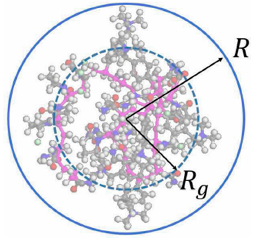
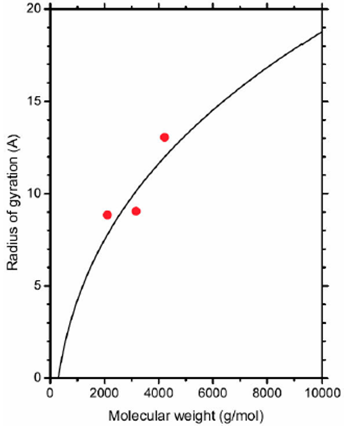
It is well known that the radius of gyration (Rg) of a polymer is proportional to a power-law of its molecular weight. As an example: Rg α Mγ, where γ ∈ (0.37, 0.43) for globular proteins [22], for cellulose [23], and γ ∈ (0.50, 0.59) for flexible polymer chains in a good solvent [24]. However, another empirical expression for the radius of gyration as a function of the molecular weight can be deduced from Fig. 2. In this case, the sphere volume with radius identical to the radius of gyration is Vg = m/ρR - ΔV, where ρR is the polymer mass density in the sphere of radius R (see Fig. 2) and ΔV is the excess volume. Thus, the new formula for the radius of gyration is
Table II Radius of gyration calculated from numerical experiments.
| Molecule | Rg (Å) |
| Polymer1 | 8.85 |
| Polymer2 | 9.05 |
| Polymer3 | 13.05 |
where M1 = 2106.8 g/mol is reported in Table I. Ag = 16.159 Å and Bg = 8.3780 Å are parameters that were determined by using the linear least square regression. Data in Table II and the fitting curve, which comes from Eq. (4), are plotted in Fig. 3. Thus, the radius of gyration as a function of the molecular weight is established.
3.2. Viscosity
Forcite uses the version of the method described by Martyna [32], where the external pressure must be isotropic, but all cell parameters (cell lengths and angles) are free to change in response to anisotropy in the internal pressure. The motion of the cell vectors, which determines the cell shape and size, is driven by the difference between the target and internal pressure, ΔP. In some cases, ΔP induces a rotational movement to the cell vectors and these movements have to be artificially suppressed. The method by Souza and Martins [34] avoids the rotational movement of the entire cell in a natural way. Souza’s method is included in the Forcite module. Thus, uniform dilatation and a fully flexible cell are combined into a hybrid method that integrates the motion equations in which a shear flow is induced in a liquid material where, additionally, the Nosé-Hoover thermostat is coupled to the above numerical integrator to preserver the thermal equilibrium [30,35], and the Berendsen method [36] is used to couple the system to a pressure bath to maintain the normal pressure.
In this third step, the molecular dynamics simulation with shear flow is
performed. The total number of steps was5 x 104, the time-step was
Δt = 1 ps, and the shear velocity was τ = 0.1/ps. The last
quantity is also known as the shear deformation rate and is the derivative of
the fluid speed in the perpendicular direction (
where V is the simulation box volume, Text = 30° C, kB is Boltzmann’s constant, and Pα,β denotes the three equivalent off diagonal elements of the (instantaneous) pressure tensor.
The relative viscosity (η* = η/ηs) is derived from the numerical experiments on the 𝔸, 𝔹 and ℂ systems, and is shown in Table III. Meanwhile, ηs is computed from the D system (brine solution without polymer). On the other hand, the polymer concentration (ρ) was calculated from the above numerical experiments and is also shown in Table III. Clearly, the polymer concentration is practically constant and ρ ≈ ρ0, where ρ0 = 0.023158 g/cm3 is the mean value. Under this consideration, the relative viscosity is approached with
where [η] is the reduced viscosity of polymer. From the Flory-Fox equation [17,18], the intrinsic viscosity of polymer ([ηi]) has the following form
where Cp is a constant that depends on the polymer molecular structure. The molecular weight M is related to the radius of gyration and was established in Eq. (4). M is solved from Eq. (4) and is substituted into Eq. (7), thus the intrinsic viscosity can be rewritten as
From this intrinsic viscosity equation, in this work, the reduced viscosity equation is proposed and has a similar structure, namely,
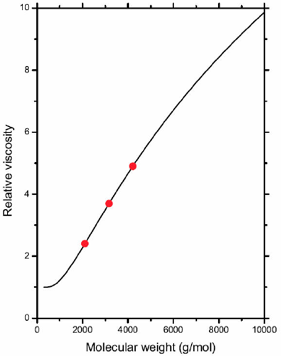
where C0 and γ0 are the adjustable parameters. In this way, Eq. (6) is used to fit the relative viscosity data shown in Table III and, therefore, C0ρ0 = 57.832 and γ0 = 5.0850 are the resulting values from the data regression. In Fig. 4, the solid curve corresponds to Eq. (6) and the solid circles are the relative viscosity data in Table III.
Table III Relative viscosity (η* = η/ηs) calculated from numerical experiments, where ηs is computed from the D system (brine solution viscosity without polymer). Polymer concentration (ρ) is in the second column.
| Molecule | ρ(g/cm3) | η* |
| Polymer1 | 0.023092 | 2.407 |
| Polymer2 | 0.023170 | 3.697 |
| Polymer3 | 0.023214 | 4.902 |
4. Experimental data
4.1. Methodology
Weighings of poly[acrylamide-co-vinylpyrrolidone-co - (vinylbenzyl) trimethylammonium]chloride powder were carried out to have concentrations of 0.001, 0.002, 0.0042, 0.005 and 0.01 g/cm3, which were dissolved in aqueous solution with 0.1 M NaCl, with soft agitation. Subsequently, the polymeric solutions were filtered with a 25 mm nylon membrane and a second membrane Millipore Millex-LCR hydrophilic with 0.45 µm to remove solid particles. The required clean solution volume in each sample was applied.
The polymeric solution was introduced into an Ostwald viscometer, pulled into the upper reservoir by suction, and then allowed to drain by gravity back into lower reservoir. In all cases, the temperature was previously fixed to 30° C with a CANNON CT-500 Series II constant temperature bath (see Fig. 5a). The time the liquid takes to pass between two etched marks, one above and one bellow the upper reservoir (see Fig. 5b), was measured. The measurements were made by triplicate for all polymeric solutions and the solvent. The time measurement of the prepared solutions (t) are shown in Table IV. The time measurement for the solvent was tsolvent = 152 s and the relative viscosity is given by ρ* = tsample / tsolvent, but the reduced viscosity [η] = (η* - 1)/η is plotted in Fig. 6. A second order polynomial equation is chosen to adjust the experimental data, namely,
Where [ηi]ρ0 = 7.7598, c1ρ20 = 18.149, and c2ρ30 = 7.6575 were found from a linear regression.
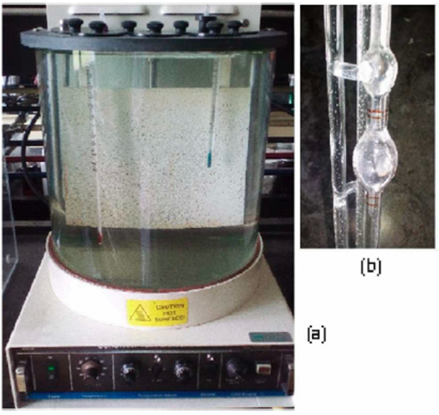
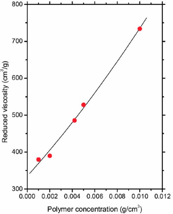
Figure 6 The solid curve corresponds to Eq. (10), and the data (solid circles) represent the reduced viscosity [η] = (η* - 1)/ρ, where η* and ρ are shown in Table IV.
Table IV Relative viscosity (η* = t=t solvent) derived from a set of experiments with different values of polymer concentration (ρ) in the fluid. The time data from Ostwald viscometer is in the second column.
| ρ(g/cm3) | t(s) | η* a |
| 0.0010 | 210 | 1.38 |
| 0.0020 | 270 | 1.78 |
| 0.0042 | 462 | 3.04 |
| 0.0050 | 553 | 3.64 |
| 0.0100 | 1267 | 8.64 |
atsolvent
The reduced viscosity measurements were performed to infer the molecular weight of the polymer. On the other hand, the theoretical framework was developed by using a set of numerical models with constant polymer concentration, namely, ρ0 = 0.023158g/cm3. Equation (10) is the starting point to find the molecular weight of the polymer and the methodology is described in the next section.
4.2. Theoretical analysis
In Eq. (9), C0 and γ0 are the parameters related to concentration ρ0. However, in a more general case, C(ρ) and γ(ρ) are functions of the concentration ρ and, therefore, C(ρ0) = C0 and γ(ρ0) = γ0. In this work, a second order polynomial is considered for both functions, namely,
where Δρ = ρ - ρ0 Clearly, the restrictions C(ρ0) = C0 and γ(ρ0) = γ0 are fulfilled. Moreover, the parameters in the following set x = {∈c1, ∈c2, ∈γ1, ∈γ2} are unknown by the moment but are determined in this section. On the other hand, the reduced viscosity given by Eq. (9) is a particular case of the following equation
In this point, Rg is a function of the polymer weight M, but in the set of experimental data in Table IV, M is constant and, therefore, Rg is considered as a parameter in this analysis. The experimental data of the reduced viscosity [η] are plotted in Fig. 6 and the points are fitted by Eq. (10). Thus, the second order Taylor expansion of Eq. (12) is
Where
Equation (10) for the reduced viscosity is the same as in Eq. (13) and therefore, the value of parameters in the set Ρ = {φ1, φ2, Rg} are determined and they are:φ1ρ0 = 0.99695, φ2ρ20 = 0.22813, and Rg = 74.194 Å. From the last value, the polymer weight can be determined. In fact, M is related to the radius of gyration Rg through Eq. (4) and, therefore, M = 2.8113 x 10⁵ g/mol is the theoretical prediction. This result of polymer weight comes from a theoretical framework that was constructed from numerical models (𝔸, 𝔹, ℂ and 𝔻), Eq. (12), which was derived from the Flory-Fox equation [17,18], and experimental measures of reduced viscosity as a function of the polymer concentration (see Table IV). On the other hand, the mean polymer weight and its molecular distribution were determined by using the Gel Permeation Chromatography (GPC) methodology. The result for the polymer weight is M(exp) ≈ 3.24 x 10⁵ g/mol. Clearly, the theoretical result underestimated the experimental value M(exp) because the polymer-polymer interactions are not included in the numerical models 𝔸, 𝔹 and ℂ.
Finally, to calculate X, the set of Eqs. (14a)-(14c) is complemented with the restriction [η]→[ηi] if ρ→0+, which is equivalent to the following two equations:
The set X is solved from Eqs. (14a), (14b), (14c), (15a) and (15b). The resulting value for the parameters in X are: εc1 ρ0 = 1.20000, εc2 ρ20 = 0.43120, εγ1 ρ0 = 0.37327, and εγ2 ρ20 = -0.03676. Thus, the reduced viscosity [η] of poly[acrylamide-co-vinylpyrrolidone-co-(vinylbenzyl) trimethylammonium]chloride is given by Eq. (12) as a function of the polymer concentration ρ in the brine and its molecular weight M.
5. Conclusions
A methodology to determine the cationic polymer weight was developed and tested. The inputs in this methodology are: 1) the mean radius of gyration R g of the polymers that are computed from the numerical experiments of poly[acrylamide - co - vinylpyrrolidone - co - (vinylbenzyl) trimethylammonium]chloride in brine; 2) the experimental results of the relative viscosity η* as a function of the polymer concentration ρ in the solution. The connection between the radius of gyration and the reduced viscosity is proposed and derived from the Flory-Fox equation for the intrinsic viscosity η*. The theoretical results of the reduced viscosity are compared to the corresponding experimental results, therefore a prediction for the polymer weight is established and given by M = 2.8113 x 10⁵ g/mol. This prediction was compared with the experimental value M(exp) ≈ 3.24 x 10⁵ g/mol derived from the GPC methodology and, perhaps, the deviation is due to the polymer-polymer interactions that are not included in the numerical models of the polymer in brine that were used in this work. Thus, the prediction of the polymer weight could be improved by enhancing the numerical models that are used to compute the radius of gyration. However, the theoretical methodology is clear and well determined.

