Research
Near-field analysis and field transformation applied to a parabolic
profile at 5 GHz
S. Peña-Ruiza
J. Sosa-Pedrozaa
F. Martínez-Zúñigaa
A. Rodríguez-Sánchezb
E. Garduño-Nolascoa
M. Enciso-Aguilara
aInstituto Politécnico Nacional, Escuela
Superior de Ingeniería Mecánica y Eléctrica. UPALM Edif. Z-4, Tercer piso, C.P.
07738 Ciudad de México.
bUniversidad de Quintana Roo Campus Chetumal.
Boulevard Bahía, Esq. Ignacio Comonfort S/N Edif. L, Col. Del Bosque, 77019.
e-mail: srgpr13@gmail.com
Abstract
We propose a method of near-field analysis and field transformation that is
applied to a 1.5 m diameter parabolic reflector at a frequency of 5 GHz. An
antenna of such dimensions requires at least a 75 m region to obtain its
radiation pattern, and this represents a problem, here arises the necessity to
make field transformations like the one presented in this work. Near field is
modeled by means of Finite Difference Time Domain Method (FDTD) and current
distribution is obtained using the discrete Pocklington equation. Radiation
pattern is calculated applying the array factor for parabolic profiles. Results
are compared with those obtained by CST Microwave Studio with a very good
agreement.
Keywords: Arrays; FDTD; Fraunhofer; modeling; parabolic profile; Rayleigh
PACS: 03.50.De; 02.70.Bf; 41.20.Jb; 07.05.Tp; 01.50.H-
Resumen
Proponemos un método para el análisis en campo cercano y transformación de campo,
que es aplicado a un reflector parabólico de 1.5 m de diámetro, a una frecuencia
de 5 GHz, una antena de tales dimensiones requiere una región de al menos 75 m
para obtener su diagrama de radiación, lo cual representa un problema, aquí es
donde surge la necesidad de realizar transformaciones de campo como la
presentada en este artículo. El campo cercano es modelado mediante el método de
Diferencias Finitas en el Dominio del Tiempo (MDFDT) y la distribución de
corriente es obtenida usando la ecuación discreta de Pocklington. El diagrama de
radiación es calculado aplicando el factor de arreglo para perfiles parabólicos.
Nuestros resultados del análisis en campo cercano y transformación de campo, son
comparados contra el modelado de la estructura en CST Microwave Studio,
encontrando muy buenas coincidencias entre ambos métodos.
Descriptores: Arreglos; MDFDT; Fraunhofer; modelado; perfil parabólico; Rayleigh
1. Introduction
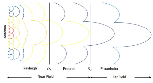
When a radiated field is distributed in space, there are three regions that identify
the process [1]: Rayleigh region, Fresnel
region and Fraunhofer region; Rayleigh region refers to the individual point field,
which means that the radiation generated at each point of the structure has not been
mixed with the other. In Fresnel region, the generated individual fields begin to
interact with each other, but their phase differences are significant, so the
radiation pattern does not have the shape that must adopt in far-field. In
Fraunhofer region, fields are added almost in phase and as they move away from the
source, the differences begin to be further reduced, so this region is referred as
the far-field region. Figure 1 describes the
three regions of the field distribution process in space. Table I shows conditions to determine the field region
distances, where D is the antenna diameter, R1 and R2 are Rayleigh and Fresnel regions and λ is the wavelength [2].
TABLE I Field regions distances.
| Antenna |
Rayleigh |
Fresnel |
Fraunhofer |
| dimension |
region |
Region |
region |
| D>>λ |
R1<λ/2π |
λ2π<R2<2D2λ
|
R2<2D2λ
|
According with Fig. 1 and Table I, the minimum distance to obtain the far-field of a 1.5 m
diameter structure, working at 5 GHz, is at least 75 m, which represents a problem
if we try to measure far-field inside a controlled environment (as in an anechoic
chamber, making nearly unmanageable to address the problem). Our method proposes to
perform a field modeling at the Rayleigh region, define virtual point currents over
the surface through discrete Pocklington equation, and then obtain far-field using
array theory; essentially a near-field to far-field transformation is carried out.
Comparing with commercial software, we reduce computational resources and the
proposed method has been used to transform near-field into far-field from real
measurements [1].
The method requires knowing the electric field near to reflector surface; this data
can be obtained from measurements as [3-6] or by field modeling in the Rayleigh region
as in [7], for this purpose, we implement a
model based on FDTD method in order to obtain the magnitude and phase of field in a
small region, near to the reflector surface. Descriptions of FDTD, discrete
Pocklington equation and parabolic array factor (PAF) are presented in following
Subsecs. 1.1 and 1.2.
1.1 Finite difference time domain method (FDTD)
The FDTD method allows analyzing the effects of electromagnetic propagation,
transforming the differential Maxwell equations into finite difference equations
that can be handled by computers [8,9]. FDTD solution involves: establish the
analysis region and divide it into cells where Maxwell’s equations are
approximated by equations in finite differences, considering all materials
within the region, using their electric and magnetic characteristics given by
their permittivity (ε), permeability (μ) and conductivity (σ); finally the iterative computing solution gives the point field
over the region.
Modeled parabolic profile was performed in two dimensions, then propagation is
restricted to the XY plane. We choose TM mode considering Ez field as the only transversal component in the XY propagating plane, therefore Ex=Ey=Hz=0. FDTD requires that the analysis region be surrounded by a free
reflection computational boundary; we choose Perfectly Matched Layer model (PML)
for our application as in [9,10]. Equations (1-4) show
the present field components.
Ezx(i,j)=abEzx(i,j)+Δtεb[Hy(i,j)-Hy(i-1,j)Δx]
(1)
Ezy(i,j)=abEzy(i,j)-Δtεb[Hx(i,j)-Hx(i,j-1)Δy]
(2)
Hx(i,j)=cdHx(i,j)-Δtμd[(Ezx+Ezy)(i.j+1)Δy-(Ezx+Ezy)(i,j)Δy]
(3)
Hy(i,j)=cdHy(i,j)+Δtμd[(Ezx+Ezy)(i+1,j)Δx-(Ezx+Ezy)(i.j)Δx]
(4)
Where:
a=1-σΔt2ε, b=1+σΔt2ε,
C=1-σ*Δt2μ, d=1+σ*Δt2μ,
As a primary source we use a standard WR187 waveguide with dimensions of 0.1×0.02215 m working at 5 GHz; as the experiment was performed in 2D, field
distribution is given by Eq. (5),
with i=j=0 at the origin and E0 constant.
Ez(i,j)n=E0sin(2πfnΔt)
(5)
1.2 Discrete Pocklington equation and parabolic array factor
The method considers that the generalized Pocklington equation [11] is valid not only on the antenna
surface, but also outside very near to it, as near as the Rayleigh region
defines it. Hence, it is possible to perform a field modeling by FDTD or by
measurement as in [1] to acquire field
points near the structure.
The current can be determined by transforming the generalized Pocklington in a
discrete form as Eq. (6)
calculating virtual currents In along the structure.
Emi=-1jωε∑n=1N[R2(k2R2-1-jkR)Sm⋅sn'+(3+3jkR-k2R2)(R⋅Sm)(R⋅sn')]e-jkR4πR5In.
(6)
Where:
Rmn=|r-r'|=[x(s)-x'(s')]2+[y(s)-y'(s')]2+[z(s)-z'(s')]2
k=Wavenumber
Solving Eq. (6) by the structure
geometry, it can be constructed a matrix as (7), where ZMN represent impedances, IN represents a virtual current to be calculated and EM represents the
modeled electric field. The matrix is solved by multiplying the electric field
vector, obtained by the FDTD modeling, by the inverse of the impedance matrix,
so vector current is obtained.
*20cZ11⋯Z1N⋮⋱⋮ZM1⋯ZMN*20cI1⋮IN=*20cE1⋮EM
(7)
Finally, far-field is calculated using the array theory [12,13] under the
assumption that calculated point currents IN in (7), represent an
array of specific elements that generate the far-field as is shown in Fig. 2. Field radiated by a parabolic array
of point sources is given by (8):
PAF(θ)=E0∑n=1N|IN|ej(kRncos(θ-ϕ)+αn)
(8)
In (8)
E0 represents the reference field of the array point sources with
unitary magnitude; the sum of the individual fields from each point antenna
considers the phase current αn, due the distance and the position of each current point Rn defined by ϕ while θ represents the angle between each point and the far-field position,
Fig. 2 describes Eq. (8).
2. Near-field analysis and far-field transformation
Table II shows the modeling parameters, where
physical dimensions are defined in meters and cells, in order to apply our
computational technique based on Pocklington equation and FDTD.
TABLE II Modeling parameters at 5 GHz.
| Units wavelength |
Cells λ
|
m 0.06 |
| Cell |
λ/20 |
0.003 |
| Calculus region Plate
diameter |
500 ×
750 500 |
1.5
× 2.25 1.5 |
| Vertex - focus |
200 |
0.6 |
| Vertex - edge |
77 |
0.23 |
| height (feeder) |
7 |
0.02215 |
| depth (feeder) |
33 |
0.1 |
| PML |
24 |
0.07 |
Calculus region dimensions are 1.5×2.25 m corresponding to 500×750 cells, considering the size of each cell as λ/20, even several authors define λ/10 is an acceptable size [9]. Our
results are compared with those of commercially available software CST, using same
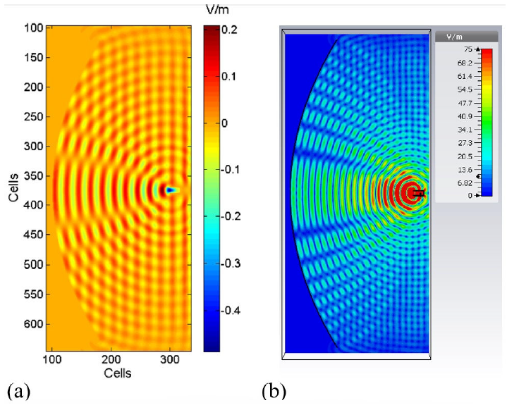
parameters for both experiments. Figure 3 shows
the calculus region and electric field distribution for both computational methods.
To have a better view of the parabolic profile, Fig. 3
(a) is shown in a smaller area defined by (90:335,95:645), where
reflector vertex is located at (100,375) and its focus at (300,375). Figure 3 displays both incident and reflected
fields, which visual comparison with CST shows a very good concordance.
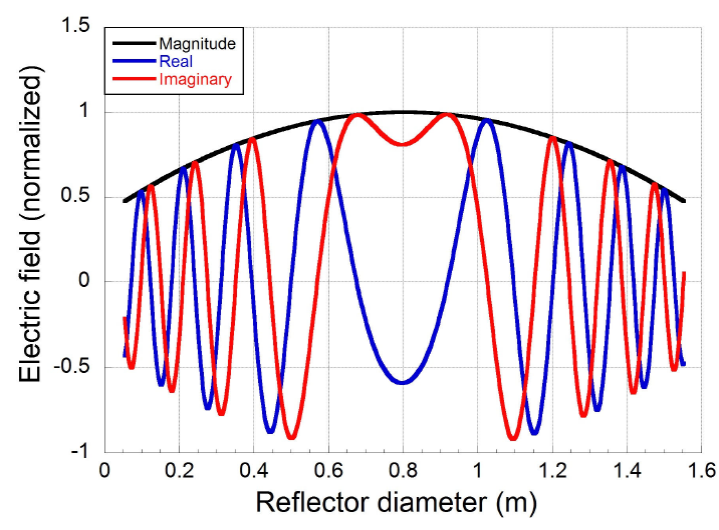
The electric field vector EM in Rayleigh region required in (6), is defined using field samples from 500 points in the FDTD matrix
at 0.003 m, one cell away from reflector surface along the parabolic profile. Figure 4 shows EM vector in magnitude, real and imaginary parts. Field phase is shown in
Fig. 5, and is obtained using distances
from reflector surface to its focus, for each field point using parabola
equation[14].
Next step in the methodology is to apply Eqs.
(6) and (7) to obtain
current along the reflector surface. Equation
(6) requires the use of parabolic geometry for distace Rmn and vectors sm and sn, that is, distances between each point of the reflector axis and each
current point [7].
Finally, the field distribution is transformed in virtual point currents along the
plate surface that will be applied in the array factor equation for the parabolic
profile (8). Figure 6, shows the magnitude, real and imaginary normalized
parts for current distribution IN. We can notice a similar behavior with electric field displayed on Fig. 4, including the 180∘ phase change of imaginary part due the reflection. Figure 7 shows the calculated phase for each current point.
Once field distribution is transformed into virtual currents along the parabolic
profile, magnitude and phase values are used in the parabolic array factor Eq. (8) to get the far-field pattern
shown in Fig. 8. As it is shown, radiation
pattern has a main lobe width of 2.5∘ which is consistent with the theory of parabolic reflectors [15], also the nearest sidelobes are observed
at -17 dB, other lobes have amplitudes between -20dB and -55 dB.
3. Comparison
In previous work [7,16], calculated radiation pattern was compared versus a
measured radiation pattern however, actual analysis allows us to observe and compare
electric field behavior with those calculated in CST to show its viability.
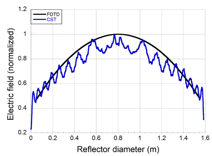
Figure 9 shows a comparison between near-field
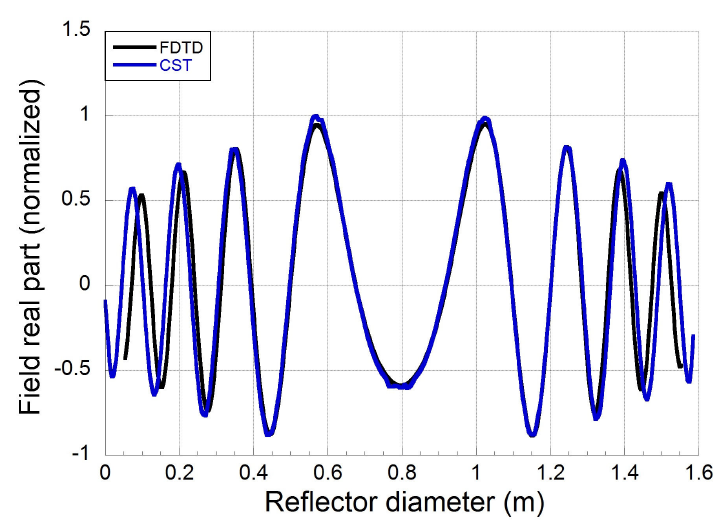
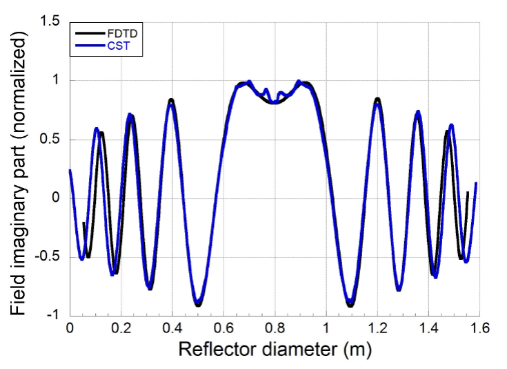
behavior for both simulations (FDTD and CST) in magnitude. Figures 10 and 11 show an
excellent agreement of the near-field in real and imaginary parts; finally,
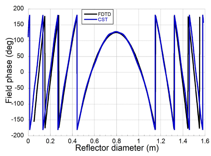
near-field phase is shown in Fig. 12, as seen
there is a clear similarity between FDTD and CST curves, specially real and
imaginary parts with small differences at the beginning and at end of curves.
Radiation patterns comparison is shown in Fig.
13, black curve represents the pattern of our method and blue curve is
the CST pattern. Similarity between both curves is evident; it can be seen that the
main lobe width is about 2.5∘ for both patterns and small differences of 5 dB at the edges (0° o 30°
and 150° to 180°).
4. Conclusions
We presented a method to transform near-field (Rayleigh region) into far-field,
without performing simulation in large computational regions, then reducing
computing resources. Even we define the field in the Rayleigh region using the FDTD
Method, an alternative proposed as future work is to measure the field near the
reflector surface and obtain far-field with Pocklington equation and Array Theory.
In addition, our method can be applied to other antenna geometries as lineal
radiators or even linear arrays or some other type of reflectors.
Comparison between our methodology (FDTD-Pocklington-PAF) and commercial software
shows that results are very similar not only for radiation pattern, but also for
near-field behavior.
Acknowledgments
The authors want to thank to the Instituto Politécnico Nacional and Consejo Nacional
de Ciencia y Tecnología of México for their support.
References
1. J. Sosa-Pedroza, L. Carrion-Rivera, F. Martínez-Zúñiga and S.
Peña-Ruiz, Una Propuesta para Transformar Mediciones de Campo Cercano en
Campo Lejano. Simposio de Metrología CENAM, México
(2014).
[ Links ]
2. Y. Huang, K, Boyle, Antennas from Theory to
Practice. (John Wiley. UK, 2008), p. 109-112.
[ Links ]
3. M. Sierra-Castañer, S. Burgos. Fresnel Zone to Far Field
Algorithm for Rapid Array Antenna Measurements. IEEE EUCAP
(2011).
[ Links ]
4. R. Cornelius, T. Salmerón-Ruiz, F. Saccardi, L. Foged, D.
Heberling, M. Sierra-Castañer, IEEE Antennas and Propagation
Magazine 56 (2014) .
[ Links ]
5. F. D’Agostino et al., IEEE Antennas and
Propagation Magazine 54 (2012).
[ Links ]
6. S. Costanzo, G. Di Massa, Microwave and Optical
Technology Letters 48 (2006).
[ Links ]
7. J. Sosa-Pedroza , M. Enciso-Aguilar, S. Peña-Ruiz, A.
Rodríguez-Sánchez, and E. Garduño-Nolasco, Microwave and Optical
Technology Letters 58 (2016).
[ Links ]
8. J. Sosa-Pedroza et al., Approach.
Electron. Lett. 47 (2011) 1308-1309.
[ Links ]
9. A. Taflove and S. C. Hagness, Computational
Electrodynamics The Finite-Diference Time-Domine Method. (Artech
House USA 2005) p. 54-75.
[ Links ]
10. M. Benavides et al., Rev. Mex. Fís.
E 57 (2011) 25-31.
[ Links ]
11. J. Sosa-Pedroza , V. Barrera-Figueroa and J. López-Bonilla,
Pocklington Equation and the Method of Moments Proc. Pakistan
Acad. (2005).
[ Links ]
12. C. A. Balanis, Antenna Theory Analysis and
Design. 3rd Ed. (John Willey, 2005) p. 284-313.
[ Links ]
13. L. Josefsson, P. Persson, Conformal Array Antenna Theory
and Design. IEEE (Press Series on Electromagnetic Wave Theory. USA,
2006), p. 15-22.
[ Links ]
14. Jacob W.M. Baars, The Paraboloidal Reflector Antenna in
Radio Astronomy and Communication. (Springer Science USA, 2007), p.
14-16.
[ Links ]
15. J. D. Kraus, R. J. Marhefka, Antennas for all
Applications. 3rd Ed. (McGraw Hill. USA, 2002), p.
564-571.
[ Links ]
16. J. Sosa, S. Peña, F. Martínez, Parabolic Reflector
Near-field to Far-field Transformation Using FDTDM and Pocklington
Equation. PIERS, (2017).
[ Links ]


 text new page (beta)
 English (pdf)
 Article in xml format
 Article references
 Send this article by e-mail
 Cited by SciELO
  Similars in
SciELO
Similars in
SciELO 
 Permalink