


 nueva página del texto (beta)
 Inglés (pdf)
 Artículo en XML
 Referencias del artículo
 Enviar artículo por email
 Citado por SciELO
  Similares en
SciELO
Similares en
SciELO 
 Permalink
1. Introduction
One can describe the geometrodynamics with the known affirmation: ’mass-energy ’tells’ spacetime how to curve and spacetime ’tells’ mass-energy how to move’ [1].
In a previous paper (G. Gomez Blanch et al, 2018), we started from the de Broglie - Bohm description of an electron trajectory [2] in the hydrogen atom. The trajectories described in the de Broglie-Bohm description belong to an Euclidian space and time. Then, we made the ansatz that this kind of trajectories, corresponding to stationary states, are geodesics of a Lorentzian manifold, so their spacetime is curved at less in the electron entourage. Moreover, an electron in a geodesic does not exert any force and does not lose energy. This fact would explain the stability of the atom, without further quantum considerations. In some way, we also established a relatioship between Quantum Theory and General Relativity.
A Lorentzial manifold has locally the structure of an Euclidian space and time, and therefore we can assimilate the de Broglie-Bohm trajectory equations with the Lorentzian geodesic equations at a differential level. In this way, we can obtain equations that interrelate the metric tensor components.
Then, we searched in the general catalogue of exact solutions of the Einstein field equations, a general metric for dust with cylindrical symmetry [3]. The selected metric model derivates from the van Stockung metric class with some contributions of other authors (King(1974); Winicour (1975); Wishweshwara -Winicour (1977)). We used this mentioned metric, but the results presented some incoherences regarding the de Broglie-Bohm approach. Then we modified this model by transforming a constant parameter into a function of the radius. We came finally over a covariant metric that was consistent with the physics, mainly regarding the velocity and the kinetic moment of the electron.
In the present paper we continue this line of work, by characterizing the relevant elements of the geometrical structure, ’that ’tells’ mass-energy the way to go’ : contravariant metric, Levi-Civita connectors, Ricci tensor and scalar curvature. We compare this scalar curvature with other geometro-dynamical approaches of the literature.
Next we consider how ’the mass-energy tells the spacetime how it wraps’. In order to do this we evaluate an element of the energy-momentum tensor: the one that represents the energy density. From it, we make experimental considerations regarding the affected volume of spacetime.
Finally, we derive a general relationship between the two components of the wave equation in space-time coordinates and the metric tensor for stationary states, and we make an interpretation of the results.
The structure of the paper goes through the phases described above: in Sec. 2 we characterize the geometric elements, discuss about the scalar curvature and compare with another geometro-dynamic interpretation; in Sec. 3 we make the derivation of the energy density component of the energy-momentum tensor and the corresponding considerations; in Sec. 4 we study the relationship between the components of the wave function of the non-relativistic quantum mechanics and the components of the metric tensor. Finally, in Sec. 5 we establish the corresponding conclusions.
2. Geometrical elements
We will describe here the general way of the geometrical calculations. We start from the covariant metrics, previously calculated (G.Gomez Blanch et al, 2018), and from there we perform the calculations of the required geometrical objects.
As it is known, the curvature of a Riemann manifold is given by the curvature tensor
where the connectors are given in function of the metric by:
and
being
2.1. The initial covariant metric
According to our previous paper (G.Gomez Blanch et alii, 2018), we start from the following metric, with
It must be highlighted that this metric for stationary states is not static, as shows the presence of not nul term
We remember briefly the deduction of this metric. We start with the geodesic equation with the proper time as parameter:
where we introduce the corresponding velocities of the de Broglie- Bohm approach in polar coordinates:
We take into acount the quantisation of the angular momentum as (u azimuthal quantum number):
If we introduce the constant
and take into account (2), the equation in the tensor metric components reads:
Here we introduce the metric form corresponding to dust particles with cylindrical symmetry that is an exact solution of the Einstein’s field equation (10):
The parameter
that can be simplified, with good approximation to:
and that has the solution:
where
2.2. Contravariant metric
We need to start from the connectors calculated according to (2) (See G.Gomez Blanch et alii, 2018). To do that, we need to calculate, in a first step, the determinant g and, from it, the contravariant metric tensor. For a metric tensor like (4), with the form:
the contravariant metric is obtained from its inverse matrix. The determinant of the covariant matrix is:
So, taking into account (4), the matrix
We substitute now the values of (5) in the previous equation, and obtain the contravariant metric tensor:
2.3. Calculation of Levi-Civita connectors
We will use the connectors of Levi -Civita, with null torsion. The reason for that election is the following. As it is known, there are two kinds of geodesics: an affin geodesic is the curve generated by a vector (i.e. the velocity) with parallel transport, and a metric geodesic that connects points by minimising their distance [5]. The Levi-Civita connection unifies the requirements for affin and metric geodesics, and therefore we use it. We need to assure that the velocity vector has parallel transport along a geodesic and therefore we need the affin connection. We also need the trajectory of the particle to be metrically coherent with the variational principle and so we need the geodesic metric.
The relationship of Levi-Civita connector with the metric is given by (2). In the calculation of the mentioned connectors we take into account the symmetry of the metric tensor and the fact that the only variable in the elements of the metric tensor is
For this calculation we want the partial derivatives of the covariant metric tensor in relation with
Next we calculate the connectors from (2). They are symmetric in their subscripts (null torsion). We obtain the following 10 generic expressions of the connectors:
Now we make the detailed calculation of these connectors, equations from (21) to (30). Those non-null ones, ordered by their upper index are:
Now we can make an additional evaluation of the proposed model. The geodesic equation (6), taking into account our previous results, reads:
If we replace the non-null values of
And regarding
In the parenthesis of the third term we easily recognize the classical ’centripetal acceleration’ and its counterpart, that cancels it. So it stands:
The second term has a very low value (some

2.4. Ricci tensor
Once the connectors are obtained, we can calculate the Ricci tensor, which allows the determination of the scalar curvature. The equation of definition reads:
and so, giving only the most significant terms,
we follow on with the calculation of the other components of the tensor, and we get:
2.5. Scalar curvature
The scalar curvature is named by the symbol R, as usual. It is calculated by the following equation:
The calculation with all elements of the Ricci tensor without approximations reads:
In our previous paper we made, for heuristic purposes, an estimation of
From this equation of the scalar curvature, we can represent
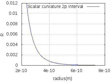
There, we can observe that:
The scalar curvature tends to 0 when
The scalar curvature takes infinite value (diverges) when the radius tends to zero. The radius
We consider now, in (53), the variation of the scalar curvature with the radial coordinate for a border limit determined by the previously mentioned selection of the constant
We can observe in this border limit, that the curvature decreases when
Beyond the upper value (
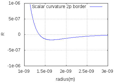
The physical meaning of that is the following one: an electron that exceeds this critical radius would get in a null curvature region and therefore would escape from the atom. If it gets in the zone where the curvature remains negative, the trajectory would also mean the exit from the atomic system, as it is represented in Fig. 3.
Therefore: if the electron gets out of the zone of positive curvature, a big alteration of its trajectory will happen. This can be the effect of an exterior physical action, that transfers energy to the atomic system. An example is the Frank-Hertz experiment, that is described by D. Bohm in the frame of his interpretation [7].
2.5.1. Comment on other evaluation of the curvature of space time in microphysical systems
Now we consider other interesting approach to our subject made by Novello, Salim and Falciano [8].
To see an approximated relationship between the quantum energy and the curvature in our model, [9] we can take the dependence of the curvature,
where
If we replace the previously mentioned approximation of R, we get:
In this point we remember the assertion of Novello, Salim and Falciano [10] that the quantum potential energy coincides with the curvature of spacetime. We must remark that this affirmation is done within the frame of an approach on Weyl’s geometry (3-D Weyl integrable space), very different of the usual Lorentzian, (pseudo-Riemannian) geometry that we use. The geometry that these authors consider has different
Indeed, according to the paper of Novello et al. [11], the relationship between the scalar curvature and the quantum potential energy would read:
very different to Equation (57). It explains that a numerical calculation in our approach yields curvature values different in some orders of magnitude respect to the corresponding to the calculations of Novello et al. [12].
Although the expression of the quantum potential energy is particularly simple in the Novello et al. approach, our approach allows us to frame our results in standard General Relativity with the use of Levi-Civita connectors, in particular respect to the Einstein field equation and the energy-momentum tensor.
2.5.2. Other scalar curvature invariants
The method used until now can be improved by using the Riemann curvature tensor to characterize the curvature in a more detailed way. Indeed, the Ricci tensor can be null and the Riemann tensor, not at all.
In connection with this, one can take into account the Kretschmann curvature, defined as:
The use of the Kretschmann scalar curvature can be considered, mainly to detect non physical singularities, as the z=0 axis, out of the nucleus entourage, and tidal effects.
So we made a first approximation to the subject. We made the calculation of the Riemann tensor
3. Considerations on the energy - momentum tensor. Volume occupied in the spacetime
The deformation of the spacetime previously considered here, derived from the de Broglie-Bohm interpretation, must have a counterpart in the energy momentum tensor. Here we are particularly interested in the correspondence with the energy term of this tensor, which is
and from there we obtain [13];
To discuss its physical meaning, we are interested in the contravariant tensor
Replacing it in the previous equation, we have:
Or as a function of the covariant Einstein tensor
Next we express the component that interest us, comparable to the energy density:
And developing it we get:
The calculation provides the following values for the components of the Einstein tensor (approximating the exponential
Making the calculation of
The
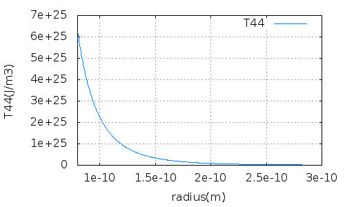
The value of the energy of the mass is
We can match the values and we have:
and therefore,
From there we obtain, always for
This calculation confirms the smallness of the affected width, of the order of
A more reasonable approximation by symmetry is that the section of this channel would be circular of radius
In Fig. 5 we represent the radius of the torus based on the radius of the trajectory of the electron.

An alternative view to the kind of spacetime deformation described above could be to consider that it has deformed all the spacetime ring between the radius
and we take
4. Relationship between the wave function and the metric tensor in the hydrogenoid atomic stationary states
We try to go deeper into the relationship between the metric tensor of an atomic hydrogenoid stationary system and the corresponding wave function, expressed with the same spacial and temporal coordinates.
We must emphasize again the different mathematical structure regarding the space and time of the de Broglie-Bohm approximation and the General Relativity. While in the de Broglie-Bohm approach we deal with the euclidean
But both models describe the same movement of the particle, at less at differential level, and we can use this to connect both mentioned approaches. So, what we intend to do is to make a coincidence between the tangent space to the manifold in the particle entourage and the space and time of the non relativistic quantum mechanics. That is mathematical coherent due to the very nature of the Lorentzial manifold[14].
To find out this relation, let us start with the de Broglie-Bohm approximation. The pilot wave that governs the movement of the electron, corresponding to the entire system, which we identify as a wave function, is given in polar form like:
where
In the de Broglie-Bohm approach, the force acting over the electron can be expressed as the gradient of the total potential, that is to say the electrical potential
where the second term of the second member is the quantum potential gradient.
The previous equation is expressed in cartesian coordinates, but must be referred to a general orthogonal reference system in order to express it in components and thus compare it with the geodesic equation.
To express the acceleration in a general orthogonal reference system we will use their corresponding Christoffel symbols
where we defined
Furthermore, concerning the second member: to build the gradient of a function
But we will use, as it is usual in such cases, an orthogonal curvilinear reference system, like the cylindrical, the spherical or the cartesian system. Then, Eq. (79) can be simplified by using the so-called scalar functions
And then the gradient of
In cylindrical coordinates we get:
We expand Eq. (77) in terms of the three-dimensional components (
Now, we will consider the relativistic side. We return to the hypothesis that an electron in an atomic quantum system and in a stationary state, describes a geodesic in the spacetime. The geodesic equation is:
If we take the proper time as a parameter, (latin indexes varying between 1 and 4,
From there we separate the equations related to the spatial coordinates (
The equation corresponding to
As
Here we use the local equivalence of the Euclidean space-time of the de Broglie-Bohm approach and the spacetime of the Lorentzial manifold, and we make the approximation to identify
Now we must take into account that, in the de Broglie-Bohm approach, the linear momentum of the particle can be expressed as a function of the gradient of the phase
that in curvilinear orthogonal coordinates can be written, according to Equation (81), as:
from there we get:
where we are using the velocity value of the de Broglie-Bohm approach to substitute it in the first member, the ’relativistic side’ of the equation. It is a good approximation taking into account the reduced value of the velocity compared with
The previous equation allows us to substitute its first term in Eq. (87) and get:
and in a more convenient and simplified form:
This expression is relevant to us in order to relate the connectors with the wave function components. But furthermore we directly want to relate the wave function and the metric tensor. For this reason, taking into account Eq. (2), we can write the explicit dependence from the metric tensor by replacing the connectors in Eq. (92)
This is the relationship between the components of the metric tensor around a stationary electron integrated into a hydrogenoid system, characterized by a potential V, and whose pilot wave or wave function is given by the components
A very important feature of that equation is to relate the metric tensor, that is of local character, with a non local entity: the quantum potential, represented by
We also note that that equation involves three systems of differential equations (
5. Main conclusions
In this article, we have developed the geometrodynamic model applied to a stationary state of the hydrogenoid atomic electron, taking into consideration General Relativity over the particle trajectory defined by the de Broglie-Bohm model, that was initiated in a previous article. We have determined the related Levi-Civita connectors, the contravariant metric tensor, the Ricci tensor and the scalar curvature. We have studied their features and structure and have determined the constant, in such a way that, beyond the experimental value of maximum extension of the corresponding orbital 2p, there will be null curvature (Minkowskian spacetime). A zone beyond the mentioned limit has been evidenced, where the curvature becomes negative and asymptotically null and therefore a zone where the electron is not allowed to be.
We also consider the relationship between the curvature and the quantum potential. Our approach allow us to consider the quantum potential, element of the Euclidean quantum mechanics, incorporated to our Relativistic approach in the geometrodynamics of the system, by the metric tensor.
We have analyzed the relationship of our approach of the quantum potential with another approach of the literature, which has a different geometrical basis (3-D Weyl integrable space).
We have also calculated the energy component of the energy momentum tensor, and we have interpreted its value with regard to the energy content, advancing a hypothesis about its relation with the path of the electron. Given the approximate numerical results, we have advanced the hypothesis that the deformation of spacetime produced by the proton-electron system implies that the volume affected by the energy density consists on a torus that would have the path of the electron in its axis.
It should be noted that the curvature of spacetime is conditioned by the action of electromagnetic interaction between the nucleus and the electron, and by the inertial and kinetic elements of the electron movement. These elements are included in the dynamic equations of the de Broglie-Bohm model that allow the path of the electron to be established (equivalent to the Hamiltonian approach to Standard Quantum Mechanics). The geometrical characterization carried out by us naturally starts from the results of that approach.
We have derived a relationship between the elemental wave function that describes the system in the classical space and time and the metric tensor, that describes it in a Lorentzial manifold. The affirmation that
The relationship found is such that, given a metric tensor induced by a trajectory, the wave function that generates it can be calculated. However, the reciprocal relationship is not possible: we can not derive the metric of the spacetime from the wave function if we do not make additional hypotheses. In our case, we have to do hypotheses regarding a cylindrical type metric of dust. In any case, a relation between the guiding character that the wave function has on the particle and the deformation of the spacetime described by the metric is obvious.
There are other approaches that have some common grounds with ours and that are commented in the Appendix.
Our study exceeds the de Broglie-Bohm’s theory as our approach establishes a dialectic relationship between particle and wave function, in contrast to the entirely preponderant role that de Broglie-Bohm’s theory gives to the wave over the particle, described in the expression ’pilot wave’: where the wave determines the movement of the particle, but the particle has no effect on the wave. On the contrary, our approach transfers to our model the interactive nature of Einstein field equations, in which the mass-energy configures the spacetime, as well as spacetime configures the movement of the mass- energy. This interaction should be, in our opinion, the cornerstone of the quantum geometrodynamics.
The global conclusion of it all is that our geometrodinamic approach to the microphysics, coming from the General Relativity and the de Broglie-Bohm interpretation, is physical and mathematicaly coherent and merits further theoretical and even experimental efforts to develop it.

