


 text new page (beta)
 English (pdf)
 Article in xml format
 Article references
 Send this article by e-mail
 Cited by SciELO
  Similars in
SciELO
Similars in
SciELO 
 Permalink
Introduction
Graphene synthesis is booming in material research and in nanotechnological applications. However, graphene synthesis is still an expensive procedure which isn’t easily reproduced. Nowadays, different techniques for producing graphene are known: mechanical exfoliation [1], epitaxial growth on SiC [2], liquid exfoliation [3] and chemical vapor deposition (CVD) [4]. The best way to get large area, good quality graphene monolayers is using the CVD synthesis method. To produce this type of graphene we need: a CVD furnace with a fast-cooling system, a mechanical vacuum pump, mass flow controllers, organic and hydrogen gases and a metal catalyzer substrate. Normally the CVD furnace comes with a temperature controller which lets you automate the temperature ramps that are needed. However, the mass flow controllers are very expensive and a power supply with the automated ramp option costs thousands of dollars. This is more expensive than the CVD furnace itself and some developing countries laboratories don’t have the budget for that kind of sophisticated equipment. Therefore, a low-cost fully automated controller is very important for small budget laboratories that want to study graphene. This automation of the mass flow controllers can also be used in other techniques different from CVD.
In this work, we design and develop a low-cost system based on an Arduino board to automate the flow ramps of the gas flows using mass flow controllers. We test our system with the results of graphene synthesis by the CVD method by comparing the Raman spectra of different graphene samples obtained using our Arduino system, the manual method and a National Instrument board.
2. System architecture
The system will control the power supply of the mass flow controllers (MFC). The power supply used is a 247-D from MKS that can control 4 channels independently. The control of each channel requires 2 signals: one that enables it and is a TTL signal, and another one that sends a voltage which is proportional to the aperture of the MFC valve. This latter voltage ranges from 0 V (minimum flow) to 5 V (maximum flow) and is linear with the flow rate.
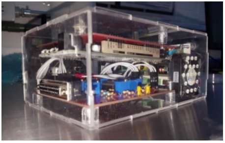
The system consists of four parts: a Simulink program which creates the flow vs. time profiles, a Labview virtual instrument that reads the Simulink flow-time data and sends it to the hardware, an Arduino board that receives the Simulink data and outputs analog signals, and a circuit that amplifies, corrects and sends the signals to the power source, which controls the mass flow controllers (MFC) through voltage changes. Figure 1 shows a photograph of the Arduino and circuit system.
The flow profiles are generated through Mathworks’ Simulink software using its signal simulation tools. Simulink’s interface allows a simple, user-friendly way to create a variety of flow patterns: constant flows, pulses, ramps, etc. A simple Matlab code allows the simulated signals to be printed in a text file with five columns: the first column contains the x value (time) of the signal, while each of the remaining columns contains the amplitude (flow rate in sccm units) of a signal. The first row of every channel has a letter that indicates whether the channel is on or off, and thus, if the communication between the MFC and the power source will be allowed.
A Labview Virtual Instrument (VI) platform, shown in the appendix, reads line by line and row by row the text file described in the previous paragraph, sending every value to the Arduino board via serial communication. In our proposed control system, the time resolution of the printed text file is one second, and as such, we are interested in maintaining the output value of the Arduino digital-to-analog-converter (DAC) during one second. Since the communication between Labview and Arduino is much faster than that, a time delay is introduced in the block diagram of the Labview VI. The resolution of the signal can be modified to be smaller, however the time it takes between Labview reading the value of a channel and Arduino “printing” it through its DAC output must be considered. Although it is possible to achieve a resolution of hundreds of milliseconds, it is not recommended since it could cause the Arduino to slow down after a while due to overwork, which would distort the flow profile. Since it is the Labview VI that controls the communication with Arduino (and therefore, the communication with the power source), it is also through this interface that the gas process is started (or stopped). The Labview interface has a display menu to select the text file which contains the flow profiles, a display menu to choose the communication port with Arduino, a “stop” button, and a graph that plots the flow rate against the elapsed time. To start the process, it is just needed to press the “Run VI” button. The graph displayed in the Labview window plots the values read from the text file, it doesn’t plot the flow (voltage) values from the circuit’s output. Because of the communication protocol used (serial) between the PC and the hardware, it is impossible to have a real-time analysis of the data, therefore, the graph is merely illustrative. However, we were able to print the pressure of the synthesis chamber which corresponds to the flow rate values given by our Arduino system.
Regarding the Arduino, the Labview VI attaches a letter at the end of every string of numbers sent through the serial port; the Arduino reads these letters to identify the channel to which the string of numbers belongs, and writes a voltage in the DAC output of the indicated channel. It must be noticed that the flow rate values in the text file must be converted to an equivalent number according to the resolution of the DAC converters of the Arduino; the maximum DAC output voltage corresponds to the highest flow rate allowed by the MFCs. This conversion is executed by the VI, so Arduino receives the voltage value in “DAC converter units”. Every time the Arduino writes a voltage in its DAC outputs, it also writes a digital high or low in one of two digital outputs (depending on the letter received from the VI). These digital signals synchronize the multiplexer and the sample & hold with the analog signals (this will be discussed later).
On the hardware side, we designed an independent four channel circuit that sends the signals received from the PC (Labview) to the MFC’s power source, shown in Fig. 2. The Arduino platform has only two boards capable of an analog output, the Arduino Zero and the Arduino Due 1, the difference between them is the number of channels (1 for the Zero and 2 for the Due) and the resolution of the converters (10 bit DAC for the Zero and 12 bit DAC for the Due). It is worth mentioning that the cost of these boards is virtually the same, therefore the choice of the Due board was straightforward 2. There are several things to be considered about the chosen board: the DAC output voltage is 0.5 V to 2.7 V, the board operating voltage is 3.3 V, and the time resolution of the system, ∆ t , is in the order of 1 µs. The complete schematic of the circuit is shown in Fig. 2, which can be divided in four general sections: demultiplexing, holding of the signal, amplifying and filtering.
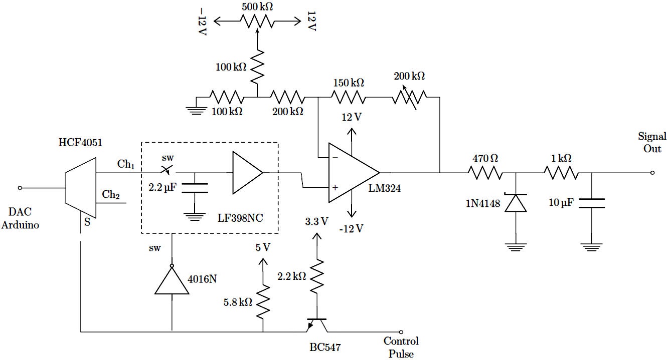
An analog circuit was used to demultiplex the Arduino signals from its 2 DACs to the four required channels. For the time being, we only use 2 signals to control 2 gases: hydrogen and methane but the system is designed to be able to control up to 4 gases. The 4 gases are needed for other material synthesis and for graphene doping. The demultiplexing could be made internally with the Arduino, but it was preferred to keep the complexity of the microcontroller script to a minimum and in consequence avoid time shifts with the computer communication. The integrated circuit used is the HCF4051, according to its datasheet its rise time is at least one order smaller than the system time resolution.
Once the signal has been demultiplexed, a sample & hold circuit (LF398) was used to keep the voltage level constant, between the assignment of the four different channels. This integrated circuit is commonly used in signal processing and is fast enough for this design. The hold capacitor was chosen carefully to avoid that its leakage current could modify the holding voltage, the typical variation was 1 mV/s. The synchronization of the multiplexer and sample & hold circuits are controlled directly from the microcontroller using standard Boolean values, but there should be special attention on what kind of logic (TTL 5 V or 3.3 V) each device is working with. The transistor, Q1, serves as a unidirectional logic voltage shifter and the NOT gate (40106), allows the syncing between the multiplexer and the sample & hold. The time delay of the NOT gate is in the order of nanoseconds, and the fact that it is a Schmitt trigger gate, makes the synchronization quite good and highly immune to noise.
For the amplification, a standard operational amplifier is used (LM324) for adjusting the output range of each channel to TTL output (0 to 5 V). The output stage consists on a protection circuit using a Zener diode with nominal voltage of 5.1 V, and a first order low pass filter. The whole circuit was powered by a low noise ±12 V power supply OJS22WX-U.
The negative voltage as well as the extra volts were used to obtain the offset and proper gain for the amplifiers. The total current drawn by the circuit is less than 100 mA. The calibration of the system (adjustment of the trimpots for gain and offset) was done when the circuit was connected directly to the MFC power source, this calibration is solely done the first time the system is powered on.
3. Application in graphene CVD synthesis
In order to test the proposed automation system, we synthesized graphene by chemical vapor deposition using different gas flow control techniques: the proposed Arduino system, directly manipulating the gas flow through the power source, that we will call the manual system and the National Instrument system. We then compared the results by their Raman spectra, using a Thermo Scientific Raman microscope with Micro-Raman using a 532 nm laser. The fingerprint of a graphene monolayer of good quality is an intense thin Lorentzian peak at 2700 cm−1 and a small thin peak at 1580 cm−1. This is due to its vibrational modes: breathing and stretching modes of the carbon atoms. For best homoge neous monolayer, the peak at 1350 cm−1 which shows defects and/or borders of the graphene film should be very small or nonexistent [5].
The three different methods of gas insertion were performed using the same recipe to be able to compare them. We used two different recipes: a continuous one and a pulsed one. The continuous recipe consists in low pressure annealing of the copper foil with 100 sccm of H2 for 70 minutes from 20oC to 1020oC and then 20 minutes with both 100 sccm of H2 and 25 sccm of CH4 at 1020oC. To control the flow through the National Instrument system, we used a Labview VI like the one used for the Arduino system. The pulsed recipe consisted in low pressure annealing of the copper foil with 100 sccm of H2 for 70 minutes from 20oC to 1020oC and then we repeated 60 times the following cycle at 1020oC: 20 seconds with both 100 sccm of H2 and 25 sccm of CH4 and 40 seconds with 100 sccm of H2 and no methane. In Fig. 3, the gas flow rates for both cases: continuous and pulsed methods are shown.

Figure 4 shows the pressure obtained at different flow rates using the Arduino system and the manual method. Both techniques show good agreement in the pressure response for each flow rate.
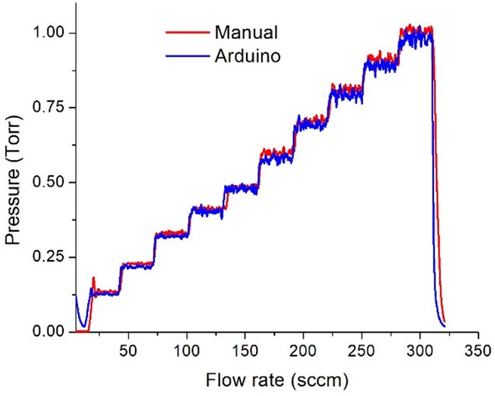
Figure 5 shows the Raman spectra for the three different methods and for both recipes, showing the graphene obtained with our Arduino method in comparison with the manual and National Instrument method. The three Raman spectra result in good quality monolayer graphene.
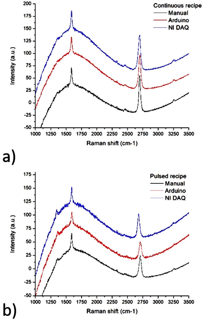
FIGURE 5 Raman spectra for graphene samples on copper using the Arduino method, the Manual method and the National Instruments for the a) continuous recipe and b) pulsed recipe.
Table I shows the 2D peak over G peak intensities ratio and D peak over G peak intensities ratio for each sample which shows that each gas insertion method gives comparable good quality graphene for both recipes. It is also shown the distance between defects, L D , for each sample obtained by the following Eq. (3) from Ref. [6]:
TABLE I Ratios between 2D and G intensities, D and G intensities and the distance between defects for each sample.
| Method | Recipe | I(2D)/I(G) | I(D)/I(G) | L D (nm) |
| Manual | Continuous | 2.2 | ∼ 0 | Too large |
| Arduino | Continuous | 2.1 | ∼ 0 | Too large |
| Nat. Ins. | Continuous | 1.9 | 0 | Too large |
| Manual | Pulsed | 1.3 | 0.3 | 22 |
| Arduino | Pulsed | 1.4 | 0.4 | 19 |
| Nat. Ins. | Pulsed | 1.6 | 0.4 | 19 |
The distance between defects, L D , is a measure of the density of point-like defects, the bigger the number, the less defects in the sample.
4. Conclusion
In summary, our Arduino system is a very good and cheap way to control the mass flow controllers for different material CVD synthesis, in particular, we have proven this for graphene monolayer samples. Our system can be used in other processes which need gas flow insertion, like sputtering or other CVD processes. The cost of the hardware part of the control circuit was less than 50 dollars, which is very low for an automation system. The results of our graphene films probed by Raman spectroscopy prove our system to be a reliable low-cost control option.


