1. Introduction

The Ginzburg-Landau equation describes the optical soliton propagation through a wide range of waveguides such as crystals, optical metamaterials, optical fibers, and optical couplers [¹-⁹]. Many powerful methods have been established to find soliton solutions of the Ginzburg-Landau equation including the modified simple equation method [¹⁰,¹¹], the semi-inverse variational principle [¹²,¹³], the extended Jacobi elliptic function expansion method [¹⁴,¹⁵], the exponential rational function [¹⁶], the generalized exponential rational function method (GERFM) [¹⁷], among others.

Due to the complex nature of the optical soliton propagation, several works consider the fractional calculus to construct new optical soliton solutions [18-21]. Nevertheless, fractional derivatives do not obey some basic properties of integer derivative such as product rule and chain rule. Recently, a local derivative called conformable derivative has been formulated by Khalil in [²²]. The conformable calculus satisfies all the properties of the standard calculus, for instance, the chain rule. This derivative can be considered to be a natural extension of the classical derivative [²³-³⁰].

Let f : [0,∞) → ℝ, the conformable derivative of a function f(t) of order α, is defined as [²²]

In this paper, the conformable GERFM is employed to study the complex time Ginzburg-Landau equation with Kerr law nonlinearity [³¹].

where Dtα is the conformable derivative of order α ∈ (0,1], x represents the non-dimensional distance across the fiber, a represents the coefficient of group velocity dispersion, and b represents the coefficient of nonlinearity. The term β arises from the perturbation effects and γ is related to the detuning effect. All above-mentioned parameters are constants real values.

2. Overview of the generalized exponential rational function method

Let us state the main steps of GERFM as follows [¹⁷]

1. Let us take into account the following nonlinear partialdifferential equation

Using the transformations Υ = Υ(χ) and χ = σx−ϕt, in nonlinear partial differential equation (3), we define attain

which is proposed as an ordinary differential equation; where the values of σ and ϕ will be determined later.

2. Consider Eq. (4) has the solution of the form

where

The values of constants p _i ,q _i (1 ≤ i ≤ 4), A ₀ ,A _k and B _k (1 ≤ k ≤ M) are determined, in such a way that solution (5) always satisfy Eq. (4). By considering the homogenous balance principle, the value of M is determined.

3. Placing Eq. (5) into Eq. (4), we give the following algebraic equation Ξ(Λ₁ ,Λ₂ ,Λ₃ ,Λ₄) = 0, in terms of Λ _i = e ^qiχ for i = 1,...,4. After setting each of the coefficients of variables in Ξ to zero, a system of nonlinear equations in terms of p _i ,q _i (1 ≤ i ≤ 4), and σ,ϕ,A ₀ ,A _k and B _k (1 ≤ k ≤ M) are generated.

4. By solving the above equations systems using any symbolic computation software, the values of p _i ,q _i (1 ≤ i ≤ 4), A ₀ ,A _k , and B _k (1 ≤ k ≤ M) are determined, replacing these values into Eq. (5) provides us the soliton solutions of Eq. (3).

3. Application

In order to find solutions of Eq. (2), the following new variables are introduced

where ν and k are the speed and frequency of the soliton, respectively; w represents the wave number of the soliton. Considering Eq. (7), we convert Eq. (2) in the following expression

from real part

and Eq. (9), from the imaginary parts.

If we apply the balance principle on the terms Θ³ and Θ” in Eq. (8), we have 3M = M + 2, so M = 1. Using Eq. (6) together with M = 1, we have

Proceeding as outlined in second section, we obtain the following sets of solutions

Set 1:

One obtains p = [−1,0,1,1] and q = [0,0,1,1], so Eq. (6) turns to

We also obtain

Placing values in Eqs. (10) and (11), yields the following solution

and

Set 2:

One obtains p = [−3,−2,1,1] and q = [1,0,1,0], so Eq. (6) turns to

We also obtain

Placing values in Eqs. (10) and (13), yields the following solution

and

Set 3: One obtains p = [2,0,1,1] and q = [−1,0,1,−1], so Eq. (6) turns to

We also obtain

Placing values in Eqs. (10) and (15), yields the following solution

and

Set 4:

One obtains p = [−3,−1,1,1] and q = [1,−1,1,−1], so Eq. (6) turns to

We also obtain

Placing values in Eqs. (10) and (18), yields the following solution

and

Set 5:

One obtains p = [1 − i,−1 − i,−1,1] and q = [i,−i,i,−i], so Eq. (6) turns to

We also obtain

Placing values in Eqs. (10) and (20), yields the following solution

and

Set 6:

One obtains p = [−2 − i,2 − i,−1,1] and q = [i,−i,i,−i], so Eq. (6) turns to

We also obtain

Placing values in Eqs. (10) and (22), yields the following solution

and

Set 7:

One obtains p = [2 − i,−2 − i,−1,1] and q = [i,−i,i,−i], so Eq. (6) turns to

We also obtain

Placing values in Eqs. (10) and (24), yields the following solution

and

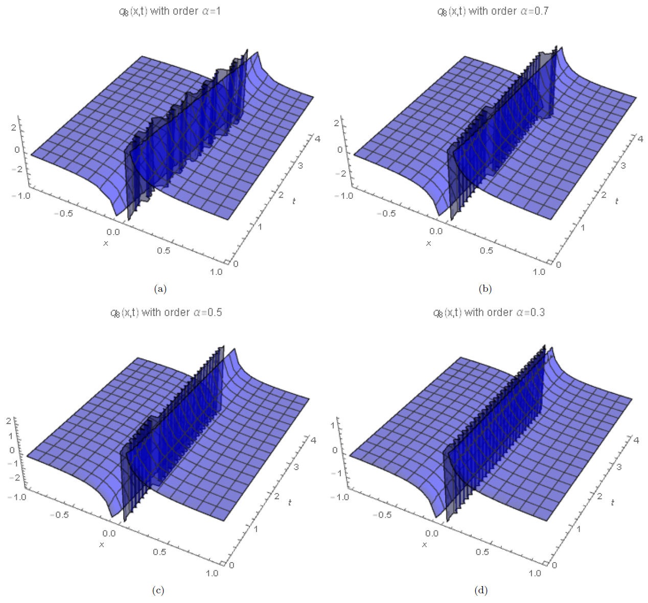
Set 8:

One obtains p = [2,0,1,−1] and q = [1,0,1,−1], so Eq. (6) turns to

We also obtain

Placing values in Eqs. (10) and (26), yields the following solution

and

Figures 1(a-d) show numerical simulations of Eq. (27) for α = 1, 0.7, 0.5, 0.3, arbitrarily chosen.

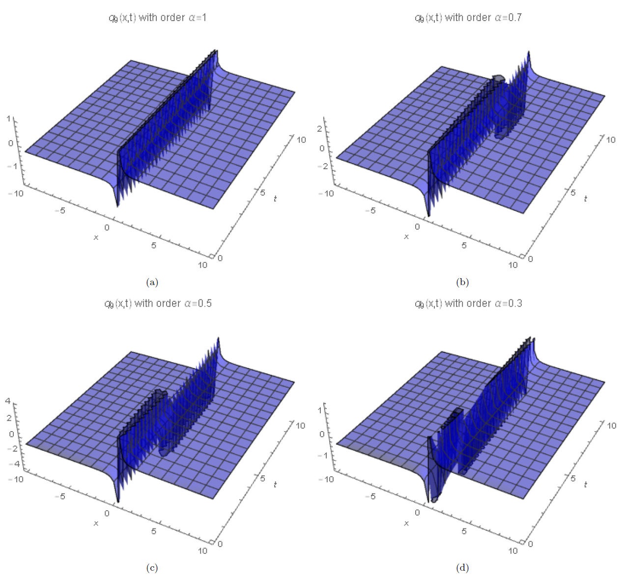
Set 9:

One obtains p = [−1,3,1,−1] and q = [1,−1,1,−1], so Eq. (6) turns to

We also obtain

Placing values in Eqs. (10) and (28), yields the following solution

and

Figures 2(a-d) show numerical simulations of Eq. (29) for α = 1, 0.7, 0.5, 0.3, arbitrarily chosen.

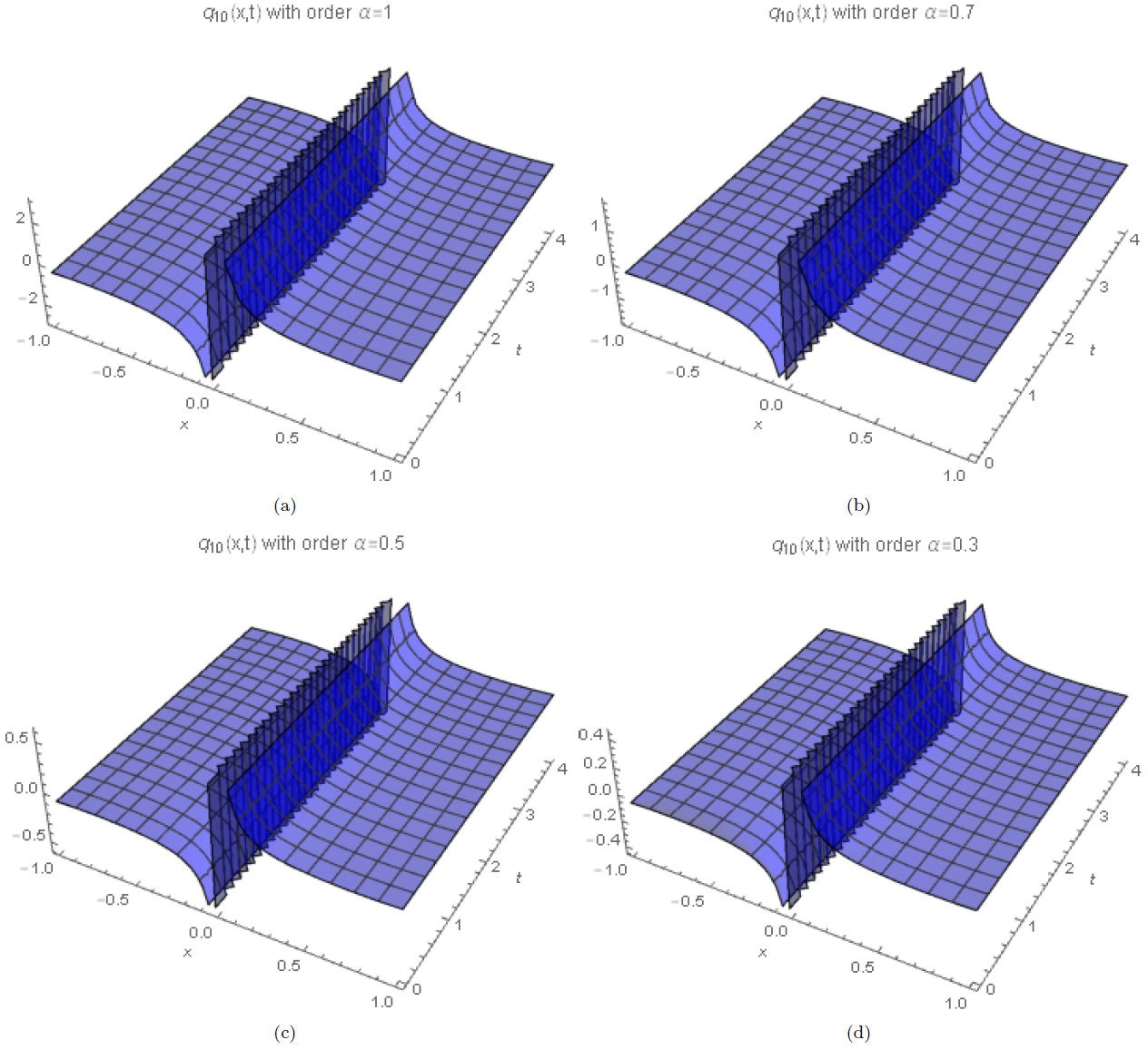
Set 10:

One obtains p = [i,−i,1,1] and q = [i,−i,i,−i], so Eq. (6) turns to

We also obtain

Placing values in Eqs. (10) and (30), yields the following solution

and

Figures 3(a-d) show numerical simulations of Eq. (31) for α = 1, 0.7, 0.5, 0.3, arbitrarily chosen.

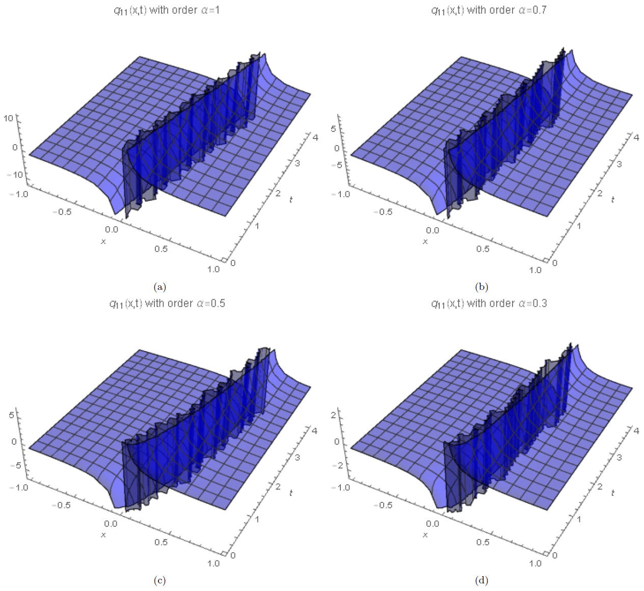
Set 11:

One obtains p = [1,1,−1,1] and q = [1,−1,1,−1], so Eq. (6) turns to

We also obtain

Placing values in Eqs. (10) and (32), yields the following solution

and

Figures 4(a-d) show numerical simulations of Eq. (33) for α = 1, 0.7, 0.5, 0.3, arbitrarily chosen.

4. Numerical simulations

In this work, we obtained different numerical solutions considering different alfa orders to obtain soliton solutions. The numerical solutions show that the change of fractional order modify the nature of the solution, and has a huge influence on the nonlinear propagation of the solitons. The analytical solutions allow graphing soliton solutions of type dark, bright, singular or combinations. Results showed that when the time derivative decreases, the amplitude of the solitons also decreases. It happens due to the decrease in velocity of the soliton, the order α characterizing the existence of the fractional structures on the system. The new analytical soliton solutions obtained in this paper have not been reported in the literature so far. Classical soliton solutions are recovered in the limit when α → 1.

5. Conclusion

In this work, we consider the generalized exponential rational function method to obtain approximate soliton solutions of the conformable Ginzburg-Landau equation with Kerr law nonlinearity. The Ginzburg-Landau equation describes the optical soliton propagation through a wide range of waveguides such as crystals, optical metamaterials, optical fibers and optical couplers. These soliton play an important and key role for information transfer via optical fibers.

The results showed that the generalized exponential rational function method is a promising approach to integrate the Ginzburg-Landau equation. We believe that this method also can be extrapolated to other nonlinear problems which arise in the theory of solitons.