


 text new page (beta)
 English (pdf)
 Article in xml format
 Article references
 Send this article by e-mail
 Cited by SciELO
  Similars in
SciELO
Similars in
SciELO 
 Permalink
1. Introduction
There are several techniques for the thermal characterization of condensed matter samples, which can be divided in two classes: Steady state and dynamical methods [1]. Among the latter one can mention the Photothermal (PT) techniques [12], which are based in the generation and detection of thermal waves. A particular type of PT technique is the one proposed in 1979 by Nordal and Kanstad for the spectroscopic analysis of solid and semi-solid materials [3], which they called Photothermal Radiometry (PTR), although a preliminary presentation was published a year earlier by these authors, for the analysis of powders [4]. The basic principle of this technique is to induce temperature changes on the sample surface by the incidence of a monochromatic modulated light beam and detect the changes produced in the thermal radiation emission. Since then, several variants of PTR technique have been reported, but its principle remains the same. Nowadays, this technique is named Modulated Photothermal Radiometry (MPTR) and, if a pulse of light replaces the exciting light beam the technique is named Pulsed Photothermal Radiometry (PPTR) [5,6]. Within the reports on the quantitative description of the modulated PTR technique, it is found that, in the eighties Santos and Miranda [7] presented a quantitative derivation of the modulated PTR production in both, frequency and time domain, using the one-dimensional model for the heat flow. From the model developed, Santos and Miranda successfully found the surface temperature fluctuation, neglecting the heat lost through the lateral walls of the sample and convection heat lost. A few years ago, Fuente et al. analyzed the ability of modulated PTR to retrieve simultaneously and accurately the optical absorption coefficient and the thermal diffusivity in homogeneous slabs [8]. Their analysis was based on considering the oscillating component of the temperature in the absence of heat losses obtained from the solution of one dimensional (1D) heat diffusion equation. Salazar et al. [9] reported the solution of 1D heat diffusion equation with non-adiabatic boundary conditions and concluded that the front and rear surface temperatures are affected by heat losses at low frequencies. Recently, Mart´ınez et al. [10] obtained a theoretical model for the PT signal in frequency domain in a 1D configuration considering convection and radiation heat losses (CRHL) in order to determine the thermal diffusivity of some low thermal conductivity materials, showing that CRHL should be taken into account for poor heat conductors at low frequencies.
The aim of this paper is to obtain analytical models closer to the physical reality for the transient thermal response in solids for application in infrared photothermal radiometry technique that takes into account the dimensions of the sample and heat losses by convection and radiation. Also, analyze the validity range of the linear approximation of the Stefan-Boltzmann’s Law, for the heat losses by thermal radiation, used in the deduction of the analytical model. This latter, by comparing results with the numerical model, obtained by means the finite element method considering the full expression of the Stefan-Boltzmann Law.
2. Theoretical Model
Consider a disc shaped sample (Fig. 1) of radius a and thickness ls that is heated by the absorption of a modulated monochromatic Gaussian beam. The generated heat flux density can be expressed as follows:
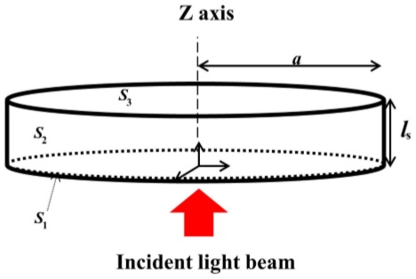
Where, I 0 and w 0 are the irradiance and the waist size of the excitation beam at the sample’s surface respectively, R s is the sample’s reflectivity, ρ is the radial cylindrical coordinate and Ψmod is a function describing the modulation. An electromagnetic-into-heat energy conversion efficiency equal to unity was assumed, as well as optical opacity of the sample. If the sample is homogenous and isotropic, then the homogenous parabolic heat diffusion equation (under cylindrical symmetry) models the heat transport, i.e.
Here, ∆T = T − T 0 is the variation of sample temperature, T, from room temperature, T 0. The solution of Eq. (2) is constrained by the following initial and boundary conditions:
In Eq. (3), F i , represents the heat flux through the ith sample surface Si(i = 1,2,3 as schematically showed in Fig. 1). Also in Eq. (3), Φcond represents the conductive heat flux, given by the Fourier heat conduction law, Φconv is the convective heat flux given by the Newton’s law of cooling, and Φrad stands for the thermal radiation flux, described by the Stefan Boltzmann law.
2.1. Analytical model
The Stefan-Boltzmann law, a non-linear expression that can be written as follows, gives the thermal radiation flux.
Where σ b is the Stefan-Boltzmann constant, and ε s is the optical emissivity of the surface, at absolute temperature T. If ∆T ¿ T 0, by expanding Φrad as a Taylor series around T 0 a linear approximation of the Stefan-Boltzmann law is obtained [2]
In this way, the boundary conditions can be rewritten as:
Here,
In Eq. (8), Θ n are the expansion coefficients of ∆T in the Fourier-Bessel orthonormal basis, defined through the set of the Bessel functions of first kind, J 0(v n r) and the associated eigenvalues, v n , are given by the roots of the next transcendental equation:
Here, Bi ρ stands for the radial Biot number. Substituting Eq. (8) into the previous Eqs. (2-6) leads to the subsequent reduced problem:
In Eq. (11), f
c
≡ α
s
· (
2.1.1. Oscillatory regime
If the modulation function Ψ mod is harmonic, then the reduced 1D-problem (Eq. (10)) can be re-written in frequency domain, using the Unitary Fourier Transform (UFT), F, leading to the following partial differential equation (PDE) problem:
The accent marks refer to the dependant variables in frequency domain. The
damping coefficients
In Eq. (16) and (17), {Cm} are the expansion coefficients of Ψmod in the Fourier basis (ω m = 2πmf). By definition, the Biot number - for a cylinder-shape sample - is related to the radial and axial Biot numbers through Eq. (18):
When the ratio
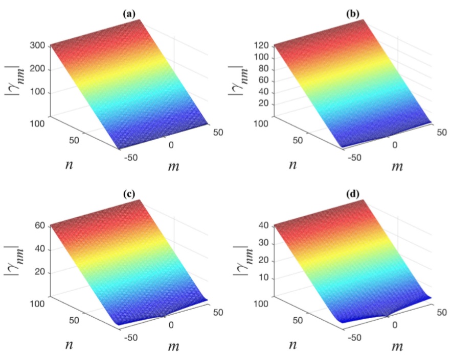
FIGURE 2 Calculated values of |γnm|for a balsa wood sample, for: (a) sf = 1, (b) sf = 0.4, (c) sf = 0.2 and (d) sf = 0.133. Here the modulation frequency was set on 100 mHz.
As can be seen from Fig. 2, by increasing the shape factor s f , the maximal magnitudes of the damping coefficients increase -from 40 to 300, for a given value of f c . The previous implies that when the shape factor increases, the lateral surface heat transfer (heat losses) increases too, and the radial heat flow through the sample tends to acquire a greater importance.
2.1.2. Transient regime
Employing the Duhamel’s Theorem [12], and considering an arbitrary -but integrable- modulation function, the solution of the 1D reduced problem, Eq. (10), is given as follows:
Where:
The Xn function stands for the stationary solution of the reduced problem, specified by the following expression:
The eigenvalues {β m }, corresponding to the eigenfunctions {Z m }, are determined by the zeros of the following transcendental equation:
This equation most be solved numerically, however, it can be demonstrated that β m ≈ mπ as long as Bi z ≪ 1. If Ψ mod is continuous and can be spanned in the Fourier basis, then the convolution product in Eq. (19) is calculated to be:
Again, {C k } are the expansion coefficients of Ψ mod in the Fourier basis. Otherwise, if Ψ mod has discontinuity points, the integral in Eq. (19) must be solved by integration by parts over the continuity subdomains.
2.2. Numerical Model
In this work, COMSOL Multiphysics (CMP) [13] has been used to solve numerically the problem described earlier in §2, by the Finite Element Method (FEM). To solve numerically Eq. (2) it is necessary to define, not only, the physical model (equations, and boundary and initial conditions), but also global parameters, the geometry (coordinate system, symmetries, physical boundaries, etc.), the material properties, and auxiliary functions (i.e. the power density distribution and the modulation function). To simulate the power density distribution in CMP, a modulated Gaussian function was defined.
In Eq. (25) Rs is the reflectivity, I
0 is the irradiance, w
0 is the laser spot radius, x and y
are the independent variables, and
In Eq. (26), ρ, C
p
and k are the mass density, the specific heat (at
constant pressure), and the thermal conductivity of the material, respectively,
In Eq. (27), the full expression of the Stefan-Boltzmann law was considered, instead of the linear approximation of the previous section, so that the boundary conditions become non-linear. For the FEM processing, a tetrahedral mesh with two different element sizes was constructed over the domain: One element size was calibrated for “general physics” with a “normal” distribution for the cylinder’s area, and the second one using a finer element distribution for both surfaces (z = 0,l s ) as showed in Fig. 3.
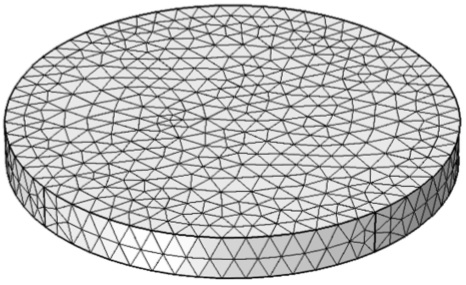
FIGURE 3 Meshing of the elements which defines the spatial domain for the numerical solution (units are not shown).
Once the model and the meshing were defined, the numerical solver was selected to generate the simulation. In this case, a direct multifrontal massively parallel sparse direct (MUMPS) solver was chosen, due to its high calculus resolution capabilities and efficient memory management in parallel computing [15]. The MUMPS solver was implemented in combination with a time stepping feature using a backward differentiation formula (BDF) [16] method in strict mode, considering second-order and fourth-order BDF to ensure a fast and accurate numerical convergence in the numerical solution of the model; obtaining a solution at the edges of the temporal subintervals, during the stipulated simulation time range. Finally, a parametric sweep was used to obtain the solutions of the model, described in the present section, at different frequencies with the same boundary and initial conditions.
3. Results and Discussion
In the present study, four different samples were considered: Two of them were low thermal conductivity balsa wood (BW) and high-density polyethylene (HDPE) materials, and the other two were high thermal conductivity cooper (Cu) and aluminium (Al) samples. The geometrical characteristics and reported physical properties of the samples are displayed in Table I [17,18].
TABLE I Geometrical and physical parameters considered for calculations.
| Sample | Material |
α ×10−3 m |
ls ×10−3 m |
εs | Rs |
αs ×10−6m2·s−1 |
ks W·m−1·K−1 |
hconv W·m−2·K−1 |
𝑓c Hz |
| M1 | BW | 5 | 1 | 0.91 | 0.20 | 0.22 | 0.11 | 4.0 | 0.070 |
| M2 | HDPE | 5 | 1 | 0.93 | 0.20 | 0.21 | 0.52 | 4.0 | 0.067 |
| M3 | Al | 5 | 1 | 0.03 | 0.96 | 93 | 238 | 4.0 | 29.61 |
| M4 | Cu | 5 | 1 | 0.05 | 0.60 | 116 | 400 | 4.0 | 36.92 |
In all cases, and for the analytical and numerical models, the modulation function Ψmod considered was the unitary rectangular wave train, with oscillation period τ mod = f −1 and wide τ mod /2, multiplied by the left-continuous unitary step function.
3.1. Analytical calculations: Oscillatory regime
The temperature distributions (surface thermograms) at ζ = 1 were calculated - using the analytical model, Eq. (10b) - for the samples defined in Table I considering, a modulation frequency, f, of 100 mHz, a value of 0.2 for the shape factor, s f , and the following values for the other input parameters: I 0 = 12.7 × 10⁴ W·m−2; σ 0 = 4.24 × 10⁻²; and T 0 = 300 K. In Fig. 4, the obtained results in temperature difference are shown at four different simulation times (0,(1/4)f −1 ,(1/2)f −1 ,(3/4)f −1).
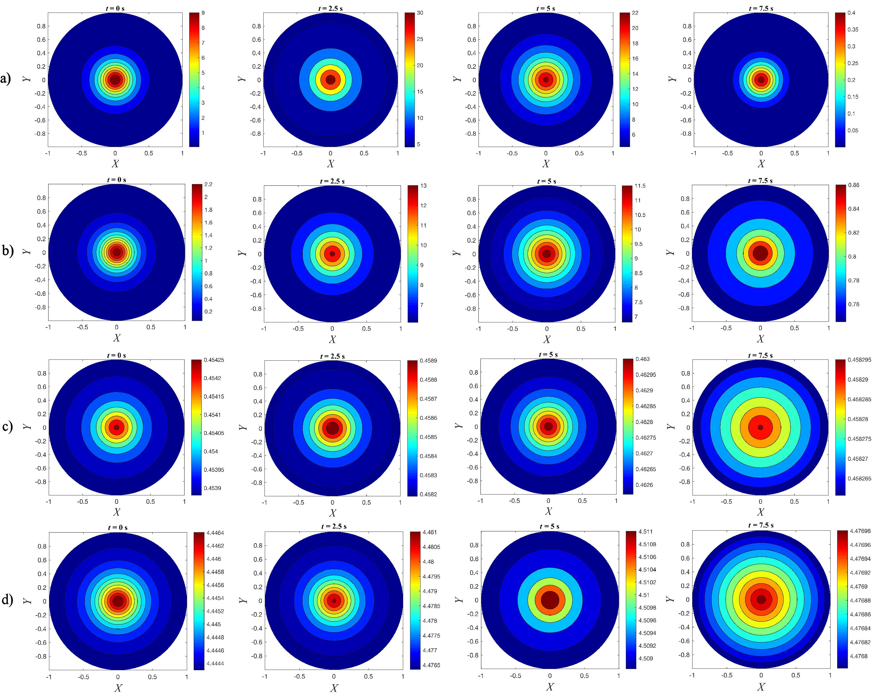
FIGURE 4 Simulated thermograms for: a) M1, b) M2, c) M3, and d) M4 samples, at four different simulation times. In each figure, 2.5 s equals f −1 /4. The units in colour bars are K.
To have a better insight on the time evolution of the radial temperature distribution, the full-width at half-maximum (FWHM) were calculated. They are shown in Fig. 5 as a function of time, and for values of 0.2 and 0.4 for the shape factor s f .
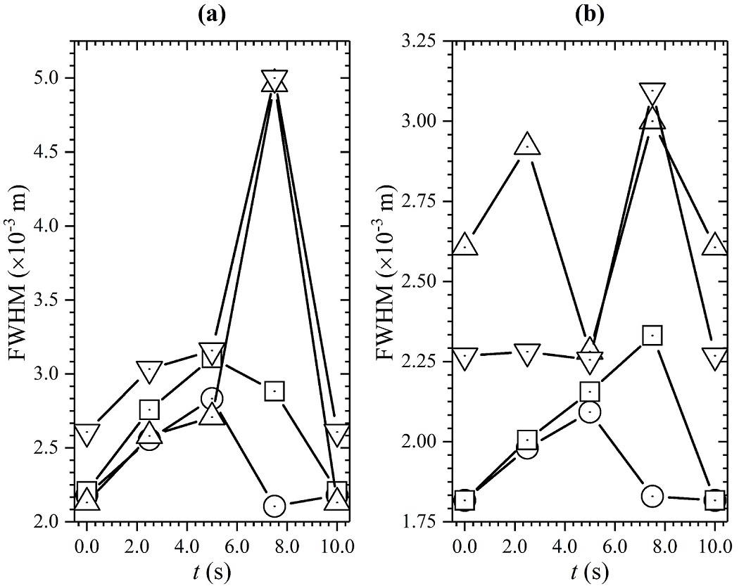
FIGURE 5 FWHM values, at different times, of: M1 (empty circles), M2 (empty squares), M3 (empty-up triangles) and M4 (empty-down triangles) samples. (a) s f =0.2 and (b) s f =0.4. In both cases f =100 mHz.
An important feature in the surface thermograms in all samples is that the radial
distribution of temperature has a Gaussian-like profile, inherit from the power
distribution. However, at t = 7.5 s (3/4 fold
τ
mod), the broadening of the radial temperature distribution covers
the hole surface in M3 and M4 samples, for the particular choice of the shape
factor s
f
= 0.2. This effect cannot be attributed solely to the
radial heat flux, but also to a combination of the magnitudes of the radial and
axial heat fluxes, and finally, to the values of Bi
p
, and
While sample M1 shows the maximal broadening at onehalf of the time period, sample M4 exhibits a significantly larger broadening in the radial distribution, reaching the maximal broadening at t = 7.5 s. This feature in the radial temperature distribution in M4 sample predicts a “homogenization” of the superficial temperature of the sample, consistent to a 1D-heat diffusion. As consequence of the particular radial distribution, the thermal wave front differs from one sample to another. This is an important issue for the analysis of the modulated photothermal radiometric signal. Taken the normalized magnitude of the spatial average |〈∆T〉|, the form of the calculated MPTR signal is clearly distinguishable for each sample (Fig. 8). As the Bi ρ decreases and f c increases, the MPTR signal becomes symmetrical. Notice also a temporal shift, due to the axial heat diffusion, and therefore, to the f c value.
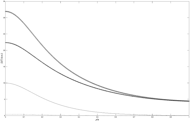
FIGURA 6 Calculated radial temperature distribution of sample M1, at: t =0 s (solid line), t =2.5 s (dash-asterisk line), t =5 s (dash-circle line) and t =7.5 s (dashed line).
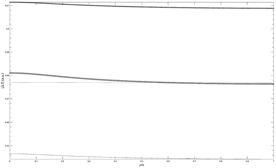
FIGURA 7 Calculated radial temperature distribution of sample M4, at: t =0 s (solid line), t =2.5 s (dash-asterisk line), t =5 s (dash-circle line) and t = 7.5 s (dashed line). For a better visualization, in this case the vertical axis is in logarithmic scale.
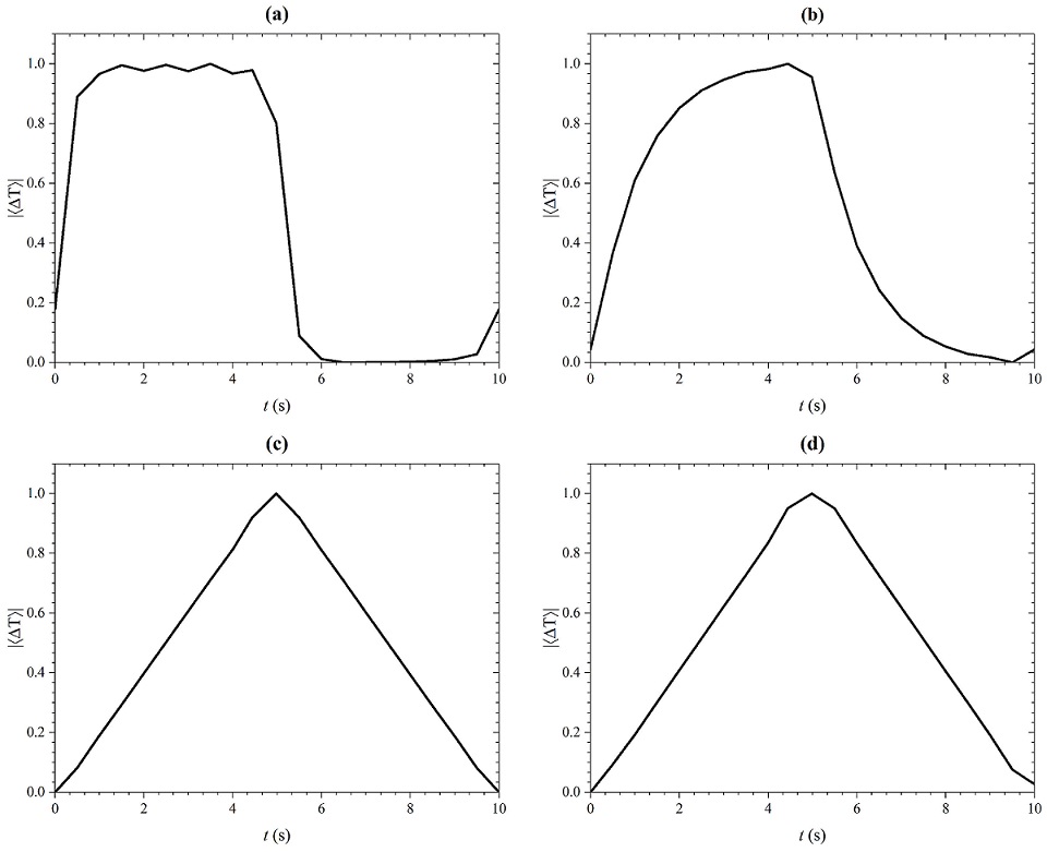
FIGURE 8 Normalized magnitude of the spatial average of the temperature oscillations of samples: (a) M1, (b) M2, (c) M3 and (d) M4. In all cases, s f =0.2 and f =100 mHz.
Naturally, the influence of other parameters must be taken into account, for
example, the magnitude of the absorbed energy flux averaged over the surface of
incidence -considered in the coefficient
3.2. Numerical calculations: Transient regime
Once that the FEM simulations were obtained to discuss the behaviour of the transient thermal response of all samples, the surface point P = (0,0,l s ) was chosen to calculate the ∆T vs. t curves. In Fig. 9, the results at P, calculated by FEM for M1 and M2 samples, are shown for f = 100 mHz. These samples, having high emissivity and low thermal conductivity, respond closely to thermally thin regime, and qualitatively alike as the thermal response described by Martínez et al. [10], analysed by using the 1D model. Next, Fig. 10 shows the ∆T vs. t curves for M3 and M4 samples, at P.
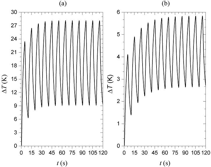
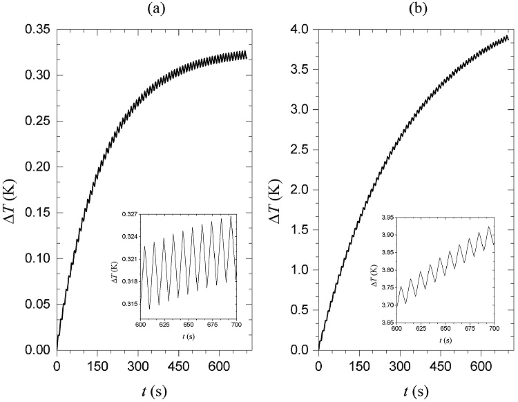
The small values of the temperature variation in samples M3 and M4 in relation to those of the samples M1 and M2 are because large values of k give small resistance to heat conduction (low values of Bi) and, therefore, small temperature gradients. This is the same reason why the predicted values of the temperature variation in sample M1 are greater than those corresponding to sample M2. Unlike this, the highest values of the temperature variation of the sample M4 with respect to those of sample M3 are due to the difference between the reflectivity values Rs of these samples (see Table I).
In Figs. 11 and 12, the amplitudes of the temperature oscillations as function of the modulation frequency, are shown for all samples, calculated by means of the analytical and numerical models.
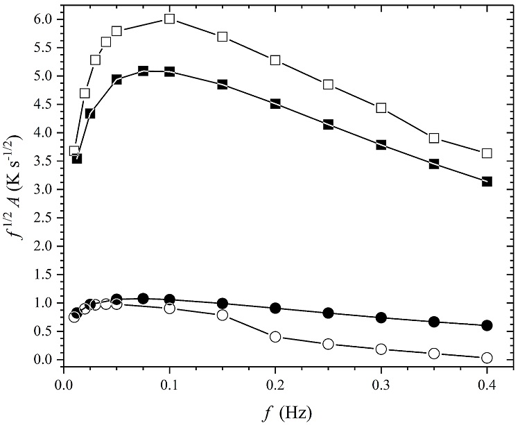
FIGURE 11 Amplitudes of the temperature variations, as function of f, for M1 sample (full circle (a), empty circle (n)), and M2 sample (full square (a), empty square (n)). Here: (a) = analytical, (n) = numerical.
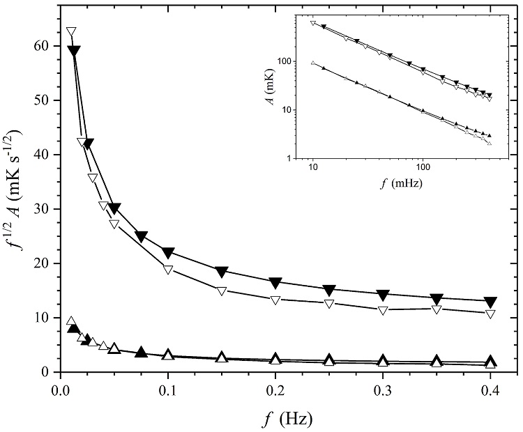
FIGURE 12 Amplitudes of the temperature variations, as function of f, for M3 sample (full up-triangle (a), empty up-triangle (n)), and M4 sample (full down-triangle (a), empty down-triangle (n)). Here: (a) = analytical, (n) = numerical.
The results of Fig. 12 show a good agreement between the analytical and numerical models for the sample M4, for which the condition ∆T ≪ T 0 is well fulfilled and the Stefan-Boltzmann law behaves with good approximation in a linear way. However, when the condition ∆T ≪ T 0 is not adequately fulfilled, the correspondence between both models is not so good, as shown by the results for samples M1, M2 y M3 in Figs. 11 and 12. In these cases, it is convenient to analyze the problem using the numerical model to obtain reliable results. On the other hand, it can be notice that M3 and M4 samples behaves almost as thermally thin samples, since the A vs. f (inset in Fig. 12) keep a f −1 dependence, unlike the behaviour of the samples M1 and M2 whose characteristic frequencies are around 5 times smaller than those of M3 and M4, see Table I.
A graph with the comparison among the numerical and analytical models with the experimental results of balsa wood and plasticine reported in Ref. [10], is shown in Fig. 13. A good agreement among them is observed, in particular, in the regions where the behavior is as a straight line the slopes are very similar, which is where the values of thermal diffusivity are obtained.
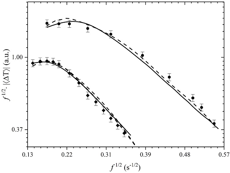
FIGURE 13 Predicted radiometric signal, calculated by analytical (solid black line), and FEM (black dashed line). Here, the full diamonds and fill circles correspond to the experimental available data for balsa wood and plasticine, respectively [10].
4. Conclusions
By solving the 2D heat diffusion equation, analytical and numerical models were obtained to describe transient and oscillatory thermal response in homogenous and finite solid samples (with cylindrical symmetry). Heat losses due to radiation and convection through front, rear and lateral surfaces were considered and a monochromatic Gaussian excitation beam that impinge on the front face of the sample. The analytical solution for the oscillatory thermal response reveals the close dependence of the thermal response on the dimensions of the sample, represented by a form factor s f , showing that when s f ≪ 1 the problem is reduced to 1D of the semi-infinite sample model. In any other case, the lateral surface heat transfer (heat losses) cannot be neglected, making its consideration necessary in a complete description of the physical situation. The results obtained for the transient thermal response are in congruence with the experimental results reported by Martínez K et al [10]. In the transient thermal response it was obtained that when the condition ∆T ≪ T 0 is well fulfilled the results obtained between the analytical and numerical models agree very well showing the utility of the Stefan-Boltzmann law linearization considered in the analytical model. However, as long as the thermal response moves away from the thermally thin regime the correspondence of the results obtained between both models becomes increasingly less, until it becomes necessary to analyze the thermal response using only the numerical model to obtain reliable results.

