Research
Local available quantum correlations for Bell diagonal states and
Markovian decoherence
H.L. Albrecht Q.a
*
D.F. Mundarainb
M.I. Caicedo S.a
a Departamento de Física, Universidad Simón
Bolívar, Apartado postal 89000, Caracas 1080, Venezuela,
b Departamento de Física, Universidad Católica
del Norte, Casilla, 1280 Antofagasta, Chile.
Abstract
Local available quantum correlations (LAQCs), as defined by Mundarain et al., are
analytically determined for Bell Diagonal states. Using the Kraus operators
formalism, we analyze the dissipative dynamics of 2-qubit LAQCs under Markovian
decoherence. This is done for Werner states under the depolarizing and phase
damping channels. Since Werner states are among those that exhibit the so called
entanglement sudden death, the results are compared with
the ones obtained for Quantum Discord, as analyzed by Werlang et al., as well as
for entanglement, i.e. Concurrence. The LAQCs quantifier only
vanishes asymptotically, as was shown to be the case for Quantum Discord, in
spite of being lower.
Keywords: Quantum correlations; quantum discord; entanglement; Bell diagonal states; Werner states; decoherence; Kraus operators
PACS: 03.65.Ud; 03.65.Yz; 03.67.Mn
1. Introduction
The study of quantum correlations is at the core of Quantum Information Theory (QIT).
Entanglement [1] had been considered to solely
encompass what Schrödinger himself esteemed to be “the
characteristic trait of quantum mechanics, the one that enforces its entire
departure from classical lines of thought” [2]. The development of Quantum Discord (QD) by Olliver and Zurek, and
independently by Henderson and Vedral [3], in
2001 showed that there are quantum correlations that are not included within the
separability criteria of entanglement. Using Werner states as an example, both
articles show that there are states that are not entangled, i.e.
null concurrence [4], and yet exhibit nonzero
QD. This has given a new impulse to a highly dynamical subfield of QIT, the study of
new quantifiers for quantum correlations.
Local measurements are the key ingredient to properly define correlations. They are
important because correlations must quantify the ability of one local observer to
infer the results of a second local observer from his own local results. The
aforementioned Quantum Discord [3]:
DA(ρAB)≡min{ΠiA}{I(ρAB)-I[(ΠA⊗1)ρAB]}=minΩ0[I(ρAB)-I(ρABcq)]
(1)
is based on comparing the quantum Mutual Information, defined for the original state ρAB as
I(ρAB)≡S(ρA)+S(ρB)-S(ρAB)
(2)
with a corresponding classical-quantum (or A-classical) state
ρABcq=∑i pi |i⟩⟨i|⊗ρBi=∑i pi Πi(A)⊗ρBi
(3)
which is a postmeasurement state in the absence of readout, where the measurement is
performed locally over the A subsystem of ρAB. Analogously, one can define DB(ρAB) comparing with a quantum-classical (or B-classical) state
ρABqc=∑i pi ρAi⊗|i⟩⟨i|=∑i pi ρAi⊗Πi(B)
(4)
Quantifiers of quantum correlations using either A-classical or B-classical states
are called Discords and are, in general, not symmetrical.
Other quantifiers [5] are based on the
difference of a quantity (e.g. mutual information, relative
entropy, etc.) with respect to systems in which both subsystems have been locally
measured. These type of states are labeled as strictly classical
ρABc=∑pij|ϕi⟩A⟨ϕi|⊗|ψj⟩B⟨ψj|
(5)
where ⟨ϕi|ϕj⟩=δij, ⟨ψi|ψj⟩=δij, ∀
i,j. It is said that there exists a local basis for which ρABc is diagonal. A special case of strictly classical states (5) worthy of
mention are product states, ρABΠ=ρA⊗ρB. For these type of states, the coefficient pij in Eq. (5) needs to be factorizable, pij=pipj. That is
ρABΠ=ρA⊗ρB=[∑pi|ϕi⟩A⟨ϕi|]⊗[∑pj|ψj⟩B⟨ψj|]=∑pipj|ϕi⟩A⟨ϕi|⊗|ψj⟩B⟨ψj|
(6)
Quantifiers of this sort include Measurement-Induced Disturbance (MID), introduced by
Luo [6], as well as its ameliorated form
(AMID), introduced by Wu et al. [7].
General quantum correlations defined in terms of local bipartite measurements were
considered recently by Wu et al. in [8], where they introduce and study non-symmetric quantum correlations
using the Holevo quantity [9] and, in a brief
final appendix, they define symmetric quantum correlations in terms of mutual
information. The LAQCs developed in [10]
focused on a slightly different version of those symmetric correlations, preserving
the requirement that any available ones must always be defined in terms of mutual
information of local bipartite measurements.
This work is focused on analytically calculating the LAQCs quantifier for the family
of BD states, given by
ρBD=141⊗1+∑ciσi⊗σi
(7)
where the coefficients ci∈[-1,1] are such that ρBD is a well behaved density matrix (i.e. has non-negative
eigenvalues) and σi are the well known Pauli matrices, and giving a first glimpse into its
dissipative dynamics. This is done by assuming Markovian decoherence and using the
Kraus operator formalism for two particular quantum channels: depolarization [11] and phase damping [12]. We will also make use of the Bloch representation for
2-qubits, given by
ρ=14(I4+x→⋅σ→⊗I2+I2⊗y→⋅σ→+T⋅σ→⊗σ→)=14(I4+∑n=13xnσn⊗I2+∑n=13ynI2⊗σn→+∑m,n=13Tnmσn⊗σm)
(8)
where {x→,y→,T} are the Bloch parameters given by xn=Tr[ρ(σn⊗I2)[, yn=Tr[ρ(I2⊗σn)[ and Tnm=Tr[ρ(σn⊗σm)[.
The present article is structured as follows: in Sec. 2 we review the main results
obtained in [10] by defining our procedure
for calculating the local available quantum correlations quantifier. Section 3 is
dedicated to the explicit calculation of this quantifier for Bell diagonal (BD)
states. We start by performing the calculation for a highly symmetrical subset of BD
states, namely Werner states. These results are then generalized for the whole BD
states family. Section 4 is devoted to the subject of Markovian decoherence. We
start by presenting the Kraus operators formalism and proceed to analyze two
dissipative quantum channels, namely depolarizing [11] and phase damping [12],
acting on the set of Werner states and determining the dissipative dynamics of the
LAQCs quantifier by means of our previous result for BD states. Finally, Sec. 5 is
devoted to the summary.
2. Local available quantum correlations for 2-qubits
A density operator ρ of a bipartite system AB can always be written in terms of different basis
ρ=∑klmnρklmn |km⟩⟨ln| = ∑ijpqRipjq |B(i,j)⟩⟨B(p,q)|
(9)
where k,l,m,n∈{0,1}, {|km⟩} is the well-known computational basis, that is, the basis of eigenvector
of σz, which is local, and {|B(i,j)⟩} is another local basis, which is equivalent under local unitary
transformations to the former one:
|B(i,j)⟩=Ua†⊗Ub†|ij⟩
(10)
Any such basis for the Hilbert space of qubits can be thought of as a new
computational basis, i.e. the basis of eigenvector of σu^≡σ→⋅u^, where σ→ is the vector whose components are the Pauli matrices and u^ is a generic unitary vector. The choosing of such direction can depend
on various conditions and / or requirements of the system at hand.
Since strictly classical states are states which are diagonal in some local basis,
one can define Xρ as the strictly classical state (5) induced by a measurement which
minimizes the relative entropy
S(ρ||Xρ)=minχρS(ρ||χρ)
(11)
where χρB given by
χρB=∑ij⟨B(i,j)|ρ|B(i,j)⟩ |B(i,j)⟩⟨B(i,j)|
(12)
and S(ρ||χ)=-Tr(ρlog2χ)-S(ρ). The minimization of such relative entropy is equivalent to finding the
optimal basis {|B(i,j)opt⟩} which will then serve as the new computational basis. Local available
quantum correlations are then defined in terms of this optimal computational
basis.
Whitout loss of generality, the search for {|B(i,j)opt⟩} can be thought of as the search for the optimal local unitary
transformations Uaop⊗Ubop such that
ρ'=Uaop⊗UbopρUaop†⊗Ubop†=∑ijpq(Rop)ipjq|ij⟩⟨pq|,i,j,p,q∈{0,1}
(13)
Therefore, analyzing the criteria for minimization of the aforementioned relative
entropy is related to the behavior of the coefficients Ropipjq. This is done by defining the most general orthonormal base (10) for
each subsystem in terms of the original computational base:
A: |μ0⟩=cosθA2|0⟩+sinθA2eiϕA|1⟩,|μ1⟩=-sinθA2|0⟩+cosθA2eiϕA|1⟩B: |ν0⟩=cosθB2|0⟩+sinθB2eiϕB|1⟩,|ν1⟩=-sinθB2|0⟩+cosθB2eiϕB|1⟩
(14)
It is important to keep in mind that this process is equivalent to finding the
unitary vectors u^A=(sinθAcosϕA,sinθAsinϕA,cosθA) and u^B=(sinθBcosϕB,sinθBsinϕB,cosθB) as to define the new σu^A⊗σu^B whose eigenvectors define the new computational basis.
In this context, Mundarain et al. define the classical correlations
quantifier as
C(ρ)=SXρ||ΠXρ
(15)
where ΠXρ is the product state (6) nearest to Xρ. As shown by Modi et al. [13], the relative entropy of a generic state,
e.g. Xρ, and its nearest product state, i.e. ΠXρ, is the total mutual information (12) of the generic state. Therefore,
the previous definition for the classical correlations quantifier may be rewritten
as:
C(ρ)=I(Xρ)
(16)
where I(Xρ) is the mutual information of the local bipartite measurement associated
with Xρ. Since the mutual information may be written as
I(ρ)=∑i,jPθ,ϕ(iA,jB) log2Pθ,ϕ(iA,jB)Pθ,ϕ(iA)Pθ,ϕ(jB)
(17)
where Pθ,ϕ(iA,jB)=⟨μi|⊗⟨νj| ρ |μi⟩⊗|νj⟩ are the probability distributions corresponding to ρAB and Pθ,ϕ(iA)=⟨μi| ρA |μi⟩, Pθ,ϕ(jB)=⟨νj| ρB |νj⟩ the ones corresponding to its marginals ρA and ρB, the required minimization of the relative entropy (11) yields a minima
for the classical correlations quantifier defined in (16). It is straightforward to
see from Eq. (13) that Pθ,ϕ(iA,jB) is directly related to Ropipjq when {|μi⟩⊗|νj⟩} is the optimal computational basis.
Once the optimal angles θ and ϕ are found and, therefore, the optimal computational basis is defined,
the state is rewritten in terms of this new basis. Since local available quantum
correlations are defined in terms of complementary basis, we are interested in
determining a new unitary vector u^⊥, contained in the plane orthogonal to our previous u^. To do so, we define a new unitary vector u^Φi for each subsystem and define the following basis:
|u0⟩(Φn)=12(|0⟩opt+eiΦn|1⟩opt),|u1⟩(Φn)=12(|0⟩opt-eiΦn|1⟩opt)
(18)
where {|0⟩opt,|1⟩opt} is the optimal computational basis and the angles Φn define a direction in the plane perpendicular to u^ for each subsystem, as to define our complementary basis [8]. In doing so, we are now able to determine
the local available quantum correlations, which are quantified in terms of the
maximal mutual information for measurements performed on σ→⋅u^Φi. That is, we compute the following probability distributions
PΦ(ia,jb,Φa,Φb)=⟨ui|⊗⟨uj| ρ |ui⟩⊗|uj⟩
(19)
and by means of (17), we determine the mutual information I(ΦA,ΦB), which is then maximized.
3. LAQCs for Bell Diagonal states
3.1 Werner States
As to better illustrate the calculation of the LAQCs quantifier, we start by
determining it for a highly symmetrical subset of BD states (7), namely Werner
states, ρw:
=z|Φ+⟩⟨Φ+|+1-z4 I4, z∈[0,1]
(20)
where z∈[0,1] and |Φ+⟩=12|0⟩|0⟩+|1⟩|1⟩ is a Bell state. Notice that (20) is obtained from (7) by setting c1=-c2=c3=z. It is well known that for these states, z<1/3 implies ρw is separable. Nevertheless, as was shown by Olliver & Zurek and Henderson & Vedral in [3], these states
have non-vanishing quantum correlations, i.e. their quantum
discord is only null for z=0.
The density matrix for the Werner states, using the standard computational
matrix, is written as:
ρw=141+z002z01-z00001-z02z001+z
(21)
By means of (14), the elements Rij (9) for the Werner states are obtained:
R00=⟨μ0|⊗⟨ν0|ρw|μ0⟩⊗|ν0⟩=14+cosθA2cosθB2sinθA2sinθB2cosϕA+ϕBz+cos2θA2cos2θB2-12cos2θA2+cos2θB2+14zR10=⟨μ1|⊗⟨ν0|ρw|μ1⟩⊗|ν0⟩=14-cosθA2cosθB2sinθA2sinθB2cosϕA+ϕBz-cos2θA2cos2θB2-12cos2θA2+cos2θB2+14zR01=⟨μ0|⊗⟨ν1|ρw|μ0⟩⊗|ν1⟩=R10R11=⟨μ1|⊗⟨ν1|ρw|μ1⟩⊗|ν1⟩=R00
(22)
Since we are using (17) to minimize (11), all that is needed are the optimal
angles {θA,θB,ϕA,ϕB}. First, we use the symmetry under exchange of subsystems A ↔ B to simplify our previous expressions using θ1=θ2=θ and ϕ1=ϕ2=ϕ. Using this, equation (22) may be written in a more compact form
as:
Rij=14[1-(-1)i+jz]-(-1)i+jsin2(θ2)×cos2(θ2)[1-cos(2ϕ)]z
(23)
where i,j∈{0,1}. In this expression we have that the first term is (1±z)/4 separated from the sector with the angular dependence. Therefore,
our optimization implies obtaining angles that minimize or even cancel out this
term for either R00=R11 or R10=R01. Analyzing the minimum of (23), it is found that this occurs for θ=ϕ=nπ as well as for θ=ϕ=n(π/2). Due to the high symmetry of Werner states, either of these choices
is consistent for obtaining the closest strictly classical state to ρw and, moreover, the density matrix for these states (20) is invariant
under (13) with either choice of θ and ϕ. Therefore, it is consistent to measure our classical correlations
in the standard computational basis, that is, for θ1=θ2=ϕ1=ϕ2=0, and Pθ,ϕ(iA,jB)=(1/4)1-(-1)i+jz and marginal probabilities Pθ,ϕ(iA)=Pθ,ϕ(iB)=(1/2). Using these expressions, the classical correlations quantifier (16)
may be written as
C(ρw)=1+z2log2(1+z)+1-z2log2(1-z)
(24)
To determine the LAQCs quantifier for the Werner states, we need to define the
complementary basis. Since we can consistently measure the classical
correlations on the Z direction, the complementary basis used will be eigenstates of σ→⋅u^, where u^ now lies in the XY plane. The probability distributions PΦ(iA,jB,ΦA,ΦB) are then determined from (19) where we also make use of the symmetry
under exchange of subsystems A ↔ B so that ΦA=ΦB=Φ, obtaining:
PΦ(0A,0B,Φ)=14[1+zcos(2Φ)]=PΦ(1A,1B,Φ)PΦ(1A,0B,Φ)=14[1-zcos(2Φ)]=PΦ(0A,1B,Φ)
(25)
where once again we have that P(0A(B))=P(1A(B))=1/2 for the marginals ρA and ρB. From these expressions it is again straightforward that the maximum
is obtained either for Φ=nπ, with n=0,1,2, or for Φ=n(π/2), with n=1,3. By means of (17), the LAQCs quantifier is then
I(ρ'w)=1+z2log2(1+z)+1-z2log2(1-z)
(26)
Therefore, we have that for Werner states, there is the same amount of classical
correlations as there are locally available quantum correlations.
3.1.1. Comparing with other quantifiers
We briefly compare our result (26) for the LAQCs quantifier with other
quantum correlations quantifiers, such as quantum discord [3] and concurrence, a quantifier for
entanglement.
It is well known that concurrencei, as introduced by Wootters [4], has a simple expression for Werner states, given by:
Cw=max0,3z-12
(27)
The expression for quantum discord for Werner states is derived from the
analytical one obtained by Luo in [14] for the more general case of BD states, given by
DBD=1-c1-c2-c34log2(1-c1-c2-c3)+1-c1+c2+c34log2(1-c1+c2+c3)+1+c1-c2+c34log2(1+c1-c2+c3)+1+c1+c2-c34log2(1+c1+c2-c3)-1-c2log2(1-c2)-1+c2log2(1+c2)
(28)
Using the fact that c1=-c2=c3=z, one can readily obtain the desired expression:
Dw=1-z4log2(1-z)-1+z2log2(1+z)+1+3z4log2(1+3z)
(29)
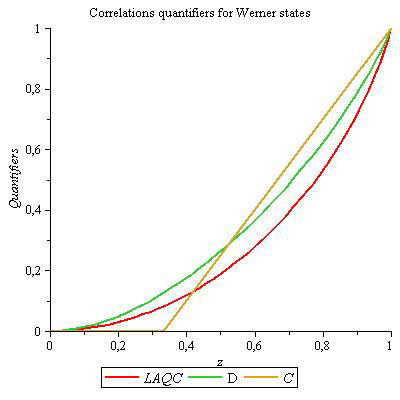
Comparison of the LAQCs quantifier with concurrence and quantum discord is
shown graphically in Fig. 1. As
observed in an example presented in [10], the quantifier for the LAQCs has values lower than the
ones for Quantum Discord. In the aforementioned case, the 2-qubit pure state |ψ⟩=cosθ|01⟩+sinθ|10⟩, written in the optimal computational basis, exhibits lower
values of the LAQCs quantifier for all values of the parameter θ, except for θ=0,π/2,π, where both quantifiers are null, and for θ=π/4,3π/4, where both are equal to 1. This same behavior is observed for
the Werner states, where both quantifiers exhibit an analogous qualitative
behavior, yet the LAQCs quntifier is almost allways lower, except for z=1, where both are null, and for z=1, where they are maximal, i.e. equal to 1.
Nevertheless, this does not imply that both quantifiers will necessarily show
in general a similar qualitative behavior. As was also pointed out in [10], for the family of mixed states ρ=p|Ψ-⟩⟨Ψ-|+(1-p)|00⟩⟨00|, numerical calculations of both QD and LAQCs quatifiers show, as
expected, that the one for LAQCs is less than the one for QD, but also that
they behave qualitatively quite differently. Moreover, in the aforementioned
work, Mundarain et al. proof that quantum-classical states have null LAQCS,
which is not necessarily the case for QD as defined in (1).
3.2. General case
We now proceed to the general case of BD states (7). Following the same procedure
as before, we determine the coefficients Rij:
R00=⟨μ0|⊗⟨ν0|ρw|μ0⟩⊗|ν0⟩=12cos(θ12)cos(θ22)sin(θ12)sin(θ22)×[cos(ϕ1-ϕ2)(c1+c2)+cos(ϕ1+ϕ2)(c1-c2)]+{cos2(θ12)cos2(θ22)-12[cos2(θ12)+cos2(θ22)]+14}c3+14=R11R10=⟨μ1|⊗⟨ν0|ρw|μ1⟩⊗|ν0⟩=-12cos(θ12)cos(θ22)sin(θ12)sin(θ22)×[cos(ϕ1-ϕ2)(c1+c2)+cos(ϕ1+ϕ2)(c1-c2)]-{cos2(θ12)cos2(θ22)-12[cos2(θ12)+cos2(θ22)]+14}c3+14=R01
(30)
Since all BD states have maximally mixed marginals, we can again make use of the
symmetry under exchange of subsystems A ↔ B, that is, θ1=θ2=θ as well as ϕ1=ϕ2=ϕ, and rewrite (30) in a more compact form as:
Rij=14[1+(-1)i+jc3]+(-1)i+j12cos2(θ2)sin2(θ2)×[(c1+c2)+cos(2ϕ)(c1-c2)-2c3]
(31)
From (31) it is straightforward to realize that {Rii,Rij}∈[0,1/2].
In this case, the minimization will depend on whether |c2|>|c3| or |c2|<|c3|, that is, on cm≡min{|c2|,|c3|}. For cm=|c2|, θ=n(π/2), with n=1,2, and ϕ=(π/2), while θ=nπ, with n=0,1,2, and ϕ=nπ, with n=0,1, for cm=|c3|. Therefore, we can write our coefficients Rij(opt) as
R00=R11=14(1+cm),R10=R01=14(1-cm)
(32)
As happened for Werner states, due to the symmetry of BD states, the density
matrix associated with (7) is invariant under the aforementioned unitary
transformations (13) for the previously chosen optimal computational basis.
Identifying Rij from (32) as our probabilities distributions Pθ,ϕ(iA,jB) and the fact that P(0A(B))=P(1A(B))=(1/2), the classical correlations quantifier (16) is then given by
C(ρw)=1+cm2log2(1+cm)+1-cm2log2(1-cm)
(33)
As previously done for the Werner states, the LAQCs quantifier is then calculated
in the basis (18), with ΦA,ΦB=Φ due to the symmetry under subsystem exchange A ↔ B, and the distribution probabilities PΦ(iA,jB,Φ) (19) are then given by:
PΦ(0A,0B,Φ)=141+c1+c22+c1-c22cos(2Φ)Pϕ(1A,0B,Φ)=141-c1+c22+c1-c22cos(2Φ)
(34)
where we also have that Pϕ(0A,0B,Φ)=Pϕ(1A,1B,Φ) and Pϕ(1A,0B,Φ)=Pϕ(0A,1B,Φ). The maximization of (34) will now depend on whether |c1|>|c2| or |c1|<|c2|, that is, it will depend on cM≡max{|c1|,|c2|}. Therefore,
cM=|c1|⇒Φ=nπ⇒PΦ(iA,jB)=14(1±c1)=14(1±cM)cM=|c2|⇒Φ=nπ2⇒PΦ(iA,jB)=14(1±c2)=14(1±cM)
(35)
where once again we have that P(0A(B))=P(1A(B))=1/2 for the corresponding marginals ρA and ρB. Taking all this into account, the LAQCs quantifier is then
I(ρw')=1+cM2log2(1+cM)+1-cM2log2(1-cM)
(36)
4. Decoherence
Modeling the behavior of any real quantum system must take into account that it will
not be completely isolated. There will be a much larger system surrounding the
quantum one, called environment, which in general will have infinite degrees of
freedom. This interaction between quantum system and environment, albeit efforts to
minimize it, will induce a process of decoherence and relaxation. This in turn may
hinder the ability of the system to maintain quantum correlations, therefore
affecting its ability to perform certain tasks in quantum computing, among others.
The study of this process can be done, under the Markovian approximation, either by
using a master equation, i.e. the Lindblad equation [15], also referred to as the
Lindblad-Kossakowski equation [16], or a
quantum dynamical semigroup approach, i.e. Kraus operator [17] formalism. In what follows we will make
use of the later, with common interactions to both subsystems, i.e.
with the interaction parameter γ equal for both subsystems so that:
ρ→ρ'=∑i,jEi⊗EjρEi⊗Ej†
(37)
Within this framework, we will study two dissipative quantum channels: Depolarizing
[11] and Phase Damping Channel [12].
4.1 Depolarizing Channel
This quantum operation represents the process of substituting an initial single
qubit state ρ with a maximally mixed one, I/2, with probability 1-γ that the qubit is left unaltered. In terms of the Bloch sphere, the
effect of this quantum channel is to uniformly contract the radius of the sphere
from 1 to 1-γ
[11]. Its Kraus operators are given
by
E0=1-3γ4I2,E1=γ2σx,E2=γ2σy,E3=γ2σz
(38)
Applying these operators on a Werner state (20) via (37), it is straightforward
to verify that the resulting density operator has the following Bloch
parameters:
xn=yn=0,∀n;T11=-T22=T33=z(1-γ)2,Tmn=0,∀m≠n
(39)
which corresponds to a Werner state where the action of this noisy quantum
channel contracts the state parameter z by a factor (1-γ)2, that is, it transforms z→z'=z(1-γ)2. We can now write both classical correlations and LAQCs quantifiers
using (24) and (26), obtaining
C(ρwDepo)=I(ρwDepo)=1+z(1-γ)22log2[1+z(1-γ)2]+1-z(1-γ)22log2[1-z(1-γ)2]
(40)
Let us now compare this with other quantum correlations quantifiers. It is well
known that Werner states exhibit entanglement sudden death (ESD) [18], as can easily be seen by using z'=z(1-γ)2 in (27):
Cw=max0,3z(1-γ)2-12
(41)
For quantum discord [3], by means of (29)
and using z→z(1-γ)2, the following expression is obtained:
Dw(Depo)=14[1-z(1-γ)2]log2[1-z(1-γ)2]-12[1+z(1-γ)2]log2[1+z(1-γ)2]+14[1+3z(1-γ)2]log2[1+3z(1-γ)2]
(42)
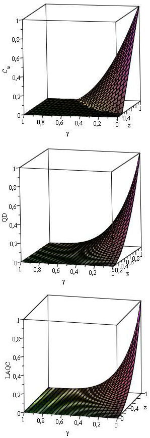
The behavior of the LAQCs quantifier, concurrence and quantum discord for a
Werner state under the action of a Depolarizing Channel is shown graphically in
Fig. 2. It is worthy noticing that,
since the resulting state of this quantum channel is still a Werner state, the
qualitative behavior of both QD and LAQCs quantifiers is indeed similar as
previously shown, maintaining the relation of the quantifier for QD being
greater than the one for LAQCs.
4.2. Phase Damping Channel
One of the quantum channels analyzed by Werlang et al. [19] in order to show the robustness of
Quantum Disord to decoherence is the Phase Damping Channel
acting on a Werner state. This noisy channel describes the loss of quantum
information without loss of energy [12].
The Kraus operators for this quantum channel are given by:
E0=1001-γ E1=000γ
(43)
Applying these operators on a Werner state (20) via (37), the resulting density
matrix has the following Bloch parameters:
xn=yn=0,∀n;T11=-T22=(1-γ)z,T33=z,Tmn=0,∀m≠n
(44)
which corresponds to a BD state (7) with c1=-c2=(1-γ)z and c3=z. Since cm=min(|c2|,|c3|)=(1-γ)z and cM=max(|c1|,|c2|)=(1-γ)z, we can now write our classical correlations and LAQCs quantifiers
using (33) and (36), obtaining
C(ρwPD)=I(ρwPD)=1+(1-γ)z2log2[1+(1-γ)z]+1-(1-γ)z2log2[1-(1-γ)z]
Even though the resulting quantum state is no longer a Werner state, since c1≠c3, we again have an equal distribution of classical and quantum
correlations. It is also noticeable that once more there is no ’sudden death’
effect observed with the LAQCs quantifier.
Concurrence for (44) is given by:
Cw(PD)=max0,z23-2γ-12
(46)
and Quantum Discord is readily obtained from (28) and (44), yielding:
Dw(PD)=1+z(3-2γ)4log2[1+z(3-2γ)]+1-z(1-2γ)4log2[1-z(1-2γ)]-1+z2log2(1+z)
(47)
The behavior of the LAQCs quantifier, quantum discord and Concurrence for a
Werner state under the action of a Phase Damping Channel is shown graphically in
Fig. 3. As can be inferred from this
graphics, the qualitative behavior of both QD and LAQCs is in this case also
quite similar, maintaining the expected relation of QD being larger than
LAQCs.
5. Conclusions
We have successfully evaluated the LAQCs quantifier for the family of BD states,
obtaining analytical formulas for it. To do so, we started with a much simpler case,
the subfamily of Werner states, as to better illustrate the procedure for
determining the LAQCs quantifier. For this subset of BD states, its behavior has
been graphically presented, comparing it with both concurrence [4] and quantum discord [3,14]. In this case QD and LAQCs
exhibit similar qualitative behavior and, as expected, the LAQCs quantifier is lower
in value than QD.
The dissipative dynamics of the 2-qubit LAQCs quantifier under Markovian decoherence
was studied for Werner states using the Kraus operators formalism in two cases:
Depolarizing channel [11] and Phase Damping
channel [12]. Analytical expressions were
obtained for both cases and presented graphically. As was previously reported for
Quantum Discord [19], LAQCs also do not
exhibit the sudden-death behavior shown by entanglement, i.e.
concurrence.
It is important to notice that we are maintaining the usual notation for Concurrence
by using the letter C and in order to distinguish it from our classical correlations
quantifier (16), we are using the subscript w to denote the Concurrence for Werner states.
References
1 R. Horodecki, P. Horodecki, M. Horodecki, K. Horodecki,
Rev. Mod. Phys. 81 (2009) 865-942.
arXiv:quant-ph/0702225.
[ Links ]
2 E. Schrödinger, Proc. Camb. Phil. Soc., 31 (1935)
555.
[ Links ]
E. Schrödinger , Proc. Camb. Phil. Soc . 32 (1936)
446.
[ Links ]
3 H. Ollivier, W. H. Zurek, Phys. Rev. Lett. 88
(2001) 017901. arXiv:quant-ph/0105072. L. Henderson, V. Vedral,
arXiv:quant-ph/0105028 (2001).
[ Links ]
4 S. Hill, W. K. Wootters, Phys. Rev. Lett. 78
(1997) 5022. arXiv:quant-ph/9703041.
[ Links ]
W. K. Wootters , Phys. Rev. Lett. 80 (1998) 2245.
arXiv:quant-ph/9709029.
[ Links ]
5 K. Modi, A. Brodutch, H. Cable, T. Paterek, V. Vedral,
Rev. Mod. Phys. 84 (2012) 1655.
arXiv:1112.6238.
[ Links ]
6 S. Luo, Phys. Rev. A 77 (2008)
022301.
[ Links ]
7 S. Wu, U. V. Poulsen, K. Mølmer, Phys. Rev. A 80
(2009) 032319. arXiv:0905.2123
[ Links ]
8 S. Wu , Z. Ma, Z. Chen, S. Xia, Sci. Rep. 4
(2014) 4036. arXiv:1301.6838.
[ Links ]
9 A. S. Holevo, Probl. Inform. Transm. 9 (1973)
177.
[ Links ]
10 D. F. Mundarain, M. L. Ladrón de Guevara, Q Inf
Proc 14 (2015) 4493-4510.
[ Links ]
11 M. Nakahara, T. Ohmi, Quantum Computing: From Linear
Algebra to Physical Realizations, (CRC Press, Boca Raton, FL,
2008), pp. 179-188.
[ Links ]
12 M. A. Nielsen, I. L. Chuang, Quantum Computation and
Quantum Information, 10th Anniversary Edition,
(Cambridge University Press, New York, NY, 2010), pp.356-385.
[ Links ]
13 K. Modi , T. Paterek , W. Son, V. Vedral , M. Williamson,
Phys. Rev. Lett. 104 (2010) 080501.
arXiv:0911.5417.
[ Links ]
14 S. Luo , Phys. Rev. A 77 (2008)
042303.
[ Links ]
15 G. Lindblad, Commun. Math. Phys. 48 (1976)
119.
[ Links ]
16 V. Gorini, A. Kossakowski, E. C. G. Sudarshan, J. Math.
Phys. 17 (1976) 821.
[ Links ]
17 K. Kraus, K., States, effects, and operations:
Fundamental notions of quantum theory - Lectures in mathematical physics at
the University of Texas at Austin, Springer Verlag (1983).
[ Links ]
K. Kraus , Ann. Phys. 64 (1971) 311.
[ Links ]
18 T. Yu, J. H. Eberly, Science 323 (2009) 598.
arXiv:0910.1396
[ Links ]
19 T. Werlang, S. Souza, F. F. Fanchini, C. J. Villas-Bôas,
Phys. Rev. A 80 (2009) 024103.
arXiv:0905.3376.
[ Links ]


 nueva página del texto (beta)
 Inglés (pdf)
 Artículo en XML
 Referencias del artículo
 Enviar artículo por email
 Citado por SciELO
  Similares en
SciELO
Similares en
SciELO 
 Permalink