


 nueva página del texto (beta)
 Inglés (pdf)
 Artículo en XML
 Referencias del artículo
 Enviar artículo por email
 Citado por SciELO
  Similares en
SciELO
Similares en
SciELO 
 Permalink
1. Introduction
The Gross-Neveu (GN) model describes a system of massless fermions with self-interacting fermions which generates a dynamical mass. The GN model was born as a toy model of Quantum Chromodynamics (QCD) 1. At first, it was studied using semiclassical functional methods, which is rigorously justified in the large N limit. In the traditional context, the GN model has shown a rich phase structure, in particular, there we have chiral symmetry breaking. Which, at first sight, it could not be allowed in 1+1 dimensions due to infrared fluctuations, unless it is invoked the large N limit 2. Despite its simplicity, it keeps many exciting features, such as discrete chiral symmetry, dynamical mass generation, and asymptotic freedom.
Curiously, this model has also application in condensed matter physics, where it describes the conductivity in some polymers. In particular, it can be mentioned the case of trans-polyacetylene, which, in a simplified continuous model, is described by the symmetric GN model 3. Besides, the massive GN model has a condensed matter analog in the modelization of polymers with non-degenerate ground states 4.
The standard approach to the GN model leads to an homogeneous condensate solution, i.e., independent of the space coordinates. After several years, it was realized that there are crystal solutions of the model, giving a rich interpretation in the realm of condensed matter physics 5. The spatial dimension could be constrained to a finite size to consider Casimir type forces. Without having in mind any particular model, we asked ourselves to consider many boundary conditions (BC’s) to simulate a broad variety of possible physical scenarios. Those are periodic, antiperiodic and confining BC’s.
Having a limited spatial extension leads us to consider the Casimir energy associated with such spaces. We found that the Casimir energies and forces are sensitive to the BC’s and parameters involved. Using the generic name of “universe" for the spatial dimension we identified the stable, metastable, attractive or repulsive regimes, depending on the parameters and BC’s we use
There is previous work in the direction we propose. In particular, in 6, it was computed the Casimir energy with MIT Bag Model boundary condition, obtaining the behavior of the Casimir energy as a function of the distance between the points and the mass of the fermionic field. On the other side, the renormalization issue of the GN model was addressed in 7, using the worldline Montecarlo approach.
In our study, we shall concentrate on the homogeneous solutions of the GN model for a
finite space of fixed size
The HF approximation implies the use of a large momentum cutoff. Since we shall deal with systems of finite spatial size, the momentum integrals must be replaced by summation on discrete modes, meaning that the natural regularization to be used is the zeta regularization technique 8.
In this work, we first ask about the ultraviolet dependence of the physical
parameters on the BC’s, considering the GN model at zero bare mass (
The second step in our work is to study the Casimir energy and force due to the
quantum fluctuation of the effective free system that arises from the HF
approximation. We consider the non-dimensional parameter
2. The Gross-Neveu Model
The Gross-Neveu Lagrangian is given by
where
In the framework of Hartree-Fock relativistic approximation, it is assumed the
expectation value
It was introduced a finite mass in order to consider a general expression and using the convention
we end up with the expression
where
From (4) we obtain a free Dirac equation
In order to obtain a stationary solution, we use the usual decomposition
Making the redefinition of the fields
we obtain a general solution
where
3. Hartree-Fock for different boundary conditions
Following the standard procedure 9, it is
possible to compute the negative energy in an infinite space taking the value of
where
Since we have a finite spatial size, the wave number
implying
where
Dealing with the summation implies a treatment of Epstein zeta function
using properties of gamma function and by means of Jacobi inverse summation formulae , we have
From the above integral, we can recognize a gamma function and a second kind Bessel function 10, leading us to the general expression
We are interested in the value
where we use tha fact that
We have the following momentum decomposition for the BC’s to be considered:
We note that the imposed boundary conditions over
Introducing the parameter of mass
As we see, the summation term can be expressed as an Epstein zeta function, so we have
Minimizing the energy density respect to
as
For the four considered BC’s, we obtained the following expressions for the energy density:
where it was introduced the non-dimensional variables
In the following step, we minimize the energy densities with respect to
where
For finite
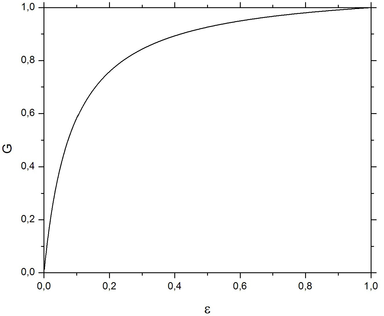
We observe from the general relation (21), that there is dependency of the constants
being
Considering the traditional point of view where the physical
For any BC, it is computed the beta function
meaning an universal behaviour of
4. Casimir Energy for global boundary conditions
Imposing BC’s of the form
In Eqs. (8) and (9) we have solutions of the form
where the values of
the constants are given by
meaning that
The BC can be expressed as
Then, the eigenvalue condition is given by
We can include the periodic and anti periodic case by the parametrization
From (8) and (9), we have
Eq. (35) leads to the condition
Since
Where
We can recognize that the summation term in (37) an Epstein zeta function, so we use the representation in (15) in order to obtain the Casimir energy. We redefine the Casimir energy given by
The Casimir Force can be obtained by the usual way
where
5. Specific boundary conditions
5.1. Periodic and Anti Periodic BC’s
The Casimir energies for the periodic and antiperiodic BC’s are given by
and the Casimir forces are
5.2. Zero current BC
The confining condition is imposing the zero current condition at the borders
In terms of components, we have
If ϕ(x)=|ϕ(x)|e α ,χ(x)=|χ(x)|e β , then
Since
The conditions are
Following the notation of (36), we have
According to Ec. (38) with
5.3. Limiting values
As can be seen from Figs. 2 and 3, the behaviour for small
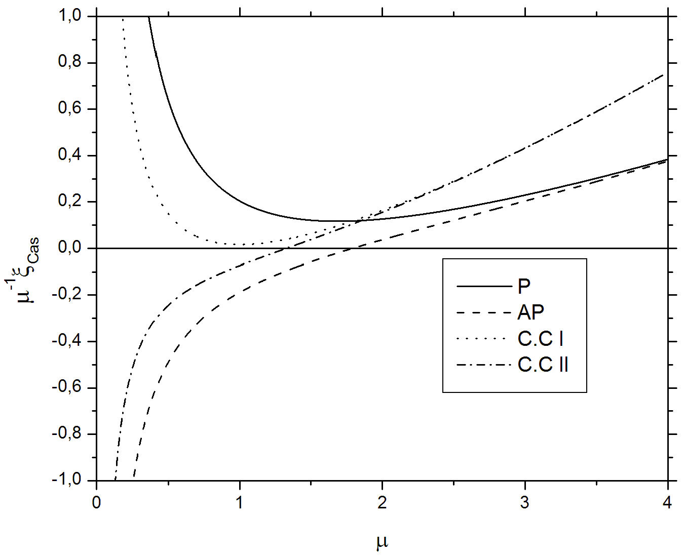
Figure 2 The

Figure 3 Behaviour of
It is more clear to take the derivative to leading order
where
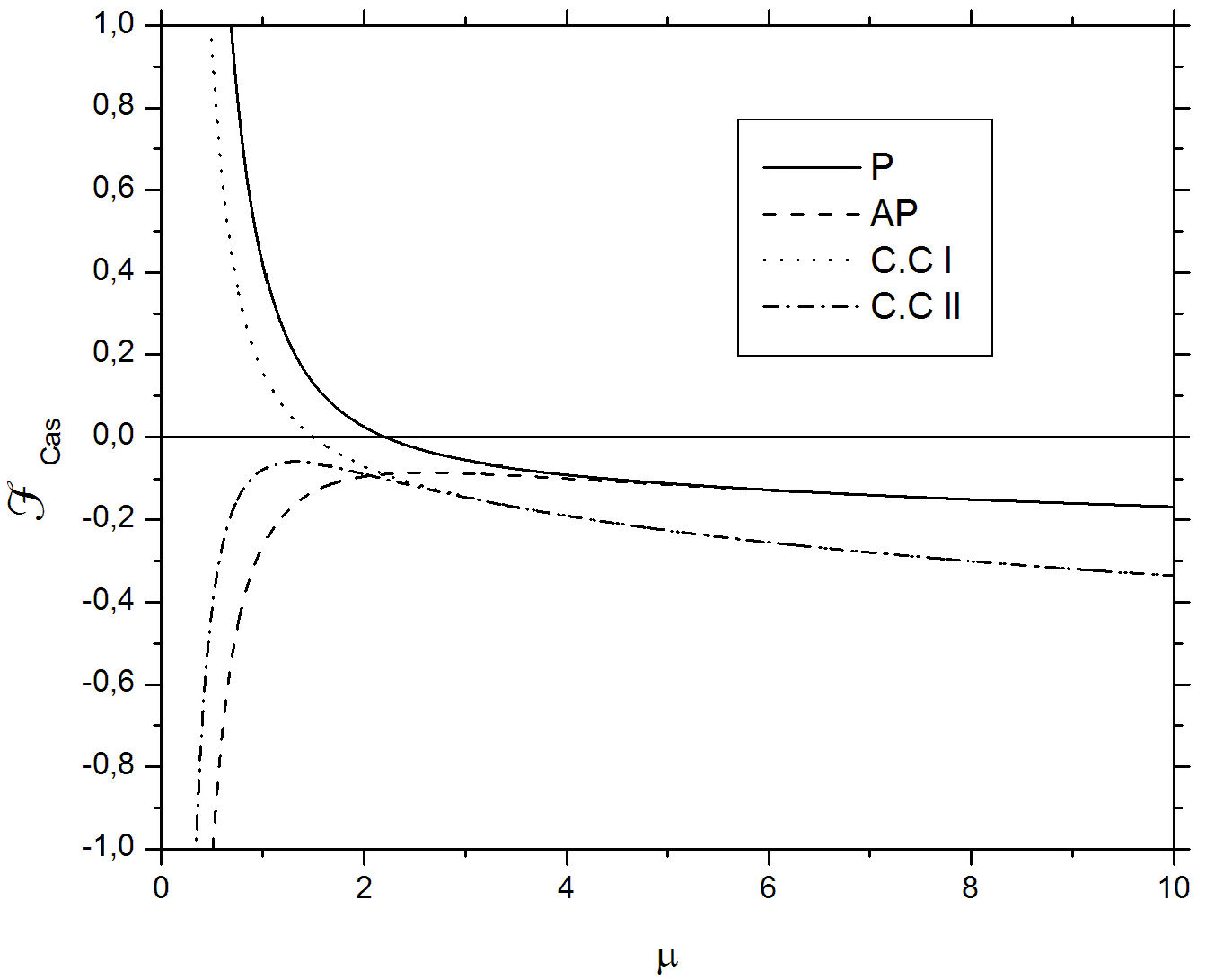
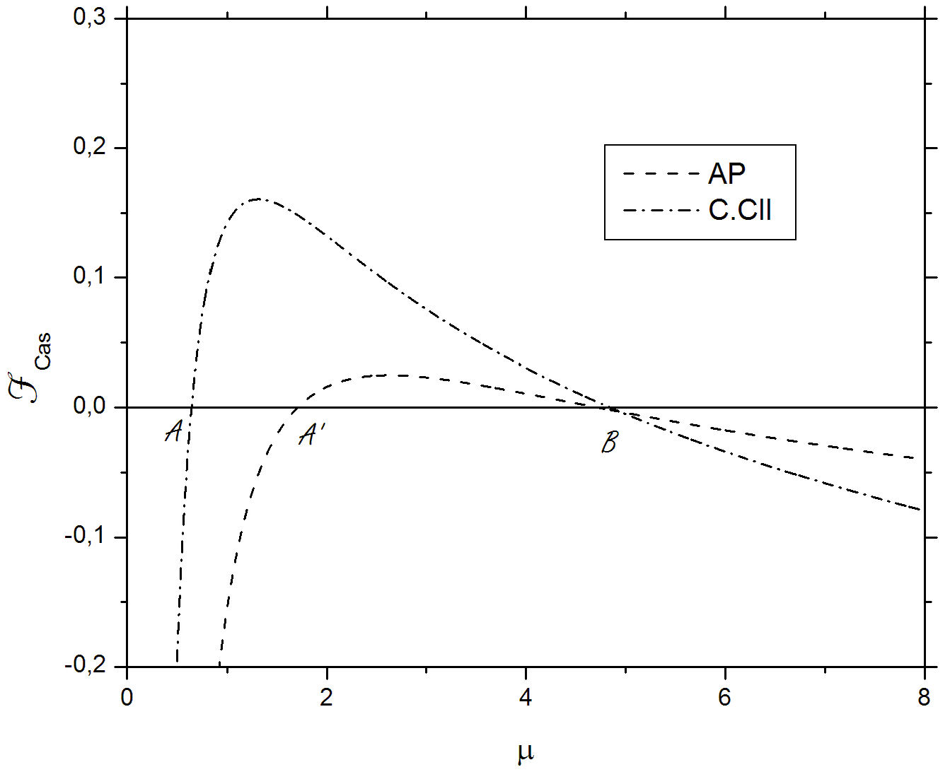
Figure 4 The
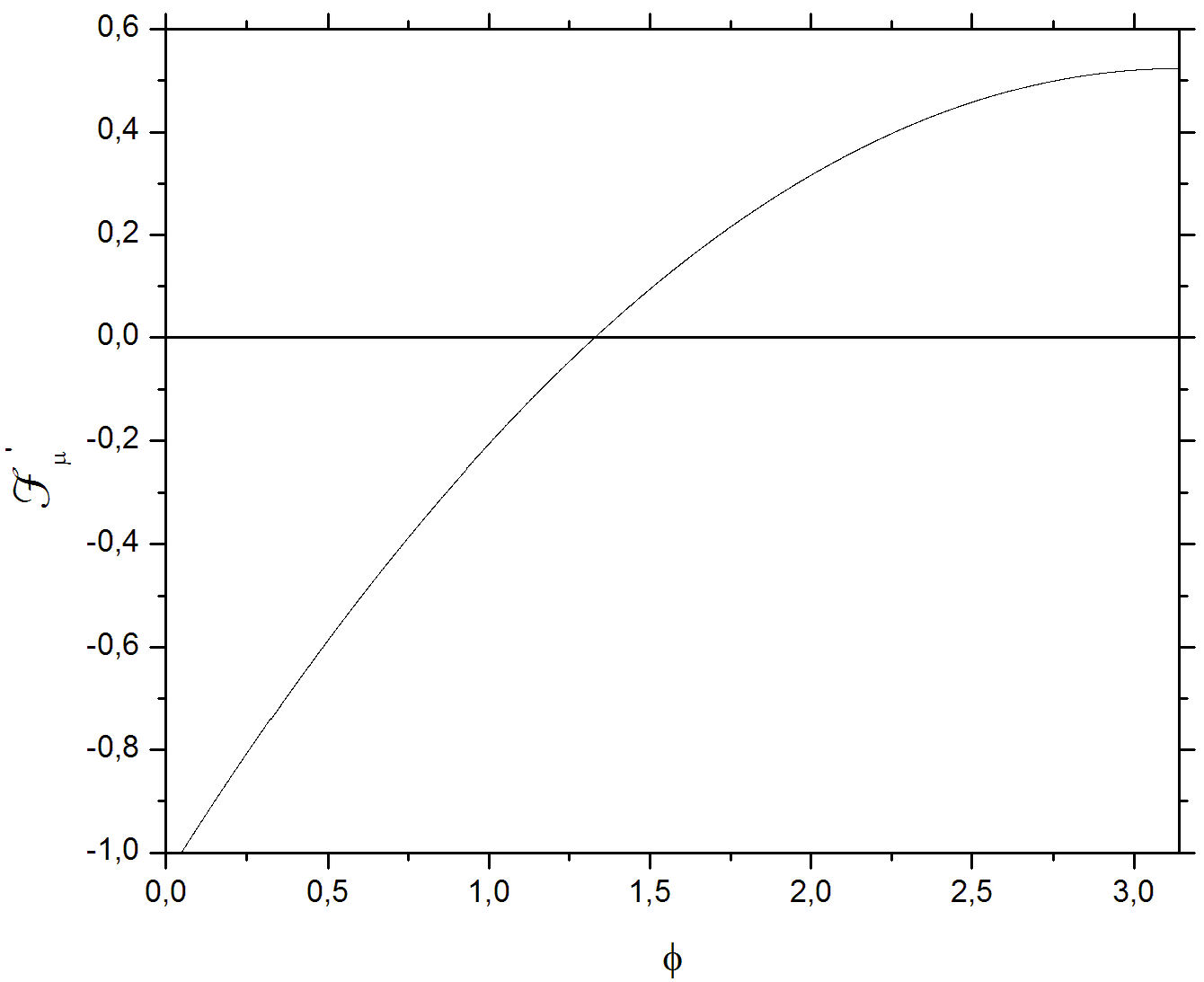
Another curious feature happen with
6. Conclusions and discussion
The first part of this article focused on the study of the ultraviolet behavior of the GN model for different BC’s, using zeta function regularization and assuming a homogeneous solution. We found that the beta function is independent of the type of boundary condition used, and that there appears a mass scale of arbitrary value. The generated dynamical mass should depend on the BC’s, if we have no prescription on the arbitrary mass scale.
Later, assuming a homogeneous solution, we studied the Casimir energy and forces for
different BC’s, if we concentrate on the behavior of
Anti periodic:
Periodic:
Confining i: The same qualitative behavior of the periodic case.
Confining ii:
We found that there is a common singular value of
For the Casimir forces, from Figs. 4 and 6, we conclude that:
Anti periodic BC:
Periodic:
Confining i: It has the same qualitative behaviour as the periodic case.
Confining ii: It has the same qualitative behaviour as the anti periodic case.
It is shown in Fig. 6 that for
From the above considerations, we conclude that for BC’s periodic and confining i,
there are two regimes of forces, being positive for “small”
For the antiperiodic and confining ii, there is a more complex situation, since its
behavior depends on the value of
This study suggests that the further natural step is to consider a general relativity study where the spatial dynamics are affected by the quantum fluctuations of the Casimir energy and confirm if the BC’s determine the existence of shrinking or expanding low dimensional universes.

