


 text new page (beta)
 English (pdf)
 Article in xml format
 Article references
 Send this article by e-mail
 Cited by SciELO
  Similars in
SciELO
Similars in
SciELO 
 Permalink
1.Introduction
Travelling reaction-diffusion waves occur in many situations of interest in chemistry, biology, physics, engineering. In some cases, such waves are isolated events, travelling independently of other chemical processes. Many chemical systems exhibit chemical waves, i.e., reactants are converted into products as the front propagates through the reaction mixture, in which autocatalytic reaction couples with molecular diffusion to give constant waveform and constant velocity fronts 1-3.
In this paper we consider reaction-diffusion travelling waves that can be initiated in a coupled isothermal chemical system governed by cubic autocatalysis. We assumed that reactions take place along semipermeable membrane interfaces with the reaction on one interface (region I). The cubic isothermal, auto-catalytic reaction step in region (I) is given by
with the step of the linear decay
where u and v are the concentrations of the reactant U and auto-catalyst V, r 1 and r 2 are the rate constants and W is some inert product of reaction. The non-dimensional equations are given by
with the boundary conditions
In the above equations we assume that cubic autocatalytic is only present in the other region II with the same rate r 1 . The two regions were considered to be coupled through a linear diffusive interchange of the auto-catalytic V. The parameters γ and k refer to the couple between the two regions and the strength of the auto-catalyst decay 4.
In fractional differentiation analysis, there are many different definitions of fractional derivatives. The Liouville- Caputo fractional derivative involve the convolution of the local derivative of a given function with power law function 5. Recently, Caputo and Fabrizio in 6, proposed a novel fractional derivative based on the exponential decay law with- out singularities 7-10. Atangana and Baleanu in 11, introduced a fractional derivative based in the Mittag-Leffler law (this function is of course the more generalized exponential function) and permits describe complex physical problems that follows at the same time the power and exponential de- cay law 12-14.
Many numerical methods for solving fractional differential equations have been developed over the past few years, such as homotopy analysis method, proposed by Liao, has been successfully applied to solving many problems in physics and engineering 15-18. The homotopy analysis method is based on construction of a homotopy which con- tinuously deforms an initial guess approximation to the exact solution of the given problem. Another powerful methods for finding exact solutions have been found in 19-24.
In this paper we obtain analytical approximate solutions to fractional cubic isothermal auto-catalytic chemical system model by applying Liouville-Caputo, Caputo-Fabrizio and Atangana-Baleanu fractional order derivatives in Liouville- Caputo sense using HATM.
2.Basic definitions
Fractional calculus unifies and generalizes the notions of integer-order differentiation. Now, we give some basic definitions and properties of FC theory.
Definition 1. The Liouville-Caputo operator (C) with order (α > 0) is defined as follows 5
For
Definition 2. The Caputo-Fabrizio fractional order derivative in the Liouville-Caputo sense (CFC) with order (α > 0) is given by 6
where M (β) is a constant of normalization that depend of β, which satisfies that, M (0) = M (1) = 1.
Definition 3. The Atangana-Baleanu fractional derivative in the Liouville-Caputo sense (ABC) with order (α > 0) is de- fined as follows 11
Where
is the Mittag-Leffler function and M (β) = M (0) = M (1) =1.
If, 0 < β ≤ 1, then we define the Laplace trans- form for the Liouville-Caputo, Caputo-Fabrizio-Caputo and the Atangana-Baleanu-Caputo fractional derivatives, respectively as follows
Considering these fractional order derivatives, we develop a new model FCIACS by replacing partial derivatives with respect to ξ by time fractional derivatives of order β.
Then the set of the Eqs. (3)-(6) become
where the operator
3.Solution of the problem
In this section, we apply the HATM 25-26 on FCIACS model. We take the initial conditions to satisfy the boundary conditions, namely
Where i=1, 2.
As we know that HAM is based on a particular type of continuous mapping 27-32
such that, as the embedding parameter q increases from 0 to 1; φi(ς, ξ; ), ψi(ς, ξ;) varies from the initial iteration to the exact solution.
Involving Eqs. (8)-(13) and 27-32 we can present the following nonlinear operators as
where Ω.(s, β) can be of type Liouville-Caputo
Caputo-Fabrizio-Caputo
and Atangana-Baleanu-Caputo
Using the embedding parameter , we develop the following set of equations
with initial conditions
where h ≠ 0 is the auxiliary parameter and H(ς, ξ) /= 0 is the auxiliary function.
Expanding in Taylor series φi(ς, ξ; ) and ψi(ς, ξ; ) with respect to
Where
If we let in Eq. (23), the series become
Considering 25-26, the m th-order deformation equation is constructed of the following manner
and
with initial conditions
Applying inverse Laplace transform, we have

4.Numerical results
In this section we evaluate the first approximations for the Liouville-Caputo, Caputo-Fabrizio-Caputo and Atangana- Baleanu-Caputo operators respectively. The intervals of convergence obtained by the h-curves, the averaged residual error, and the residual error function were evaluated. Further- more, we will show the behavior of the HATM solutions for different values of fractional derivative β.
We take the initial approximation as
For j = 1, we obtain the first approximation as following
We can obtain the first approximation via Liouville-Caputo, Caputo-Fabrizio-Caputo and Atangana-Baleanu-Caputo operators, with ΩC (s, β), ΩCF C (s, β) and ΩABC (s, β), re- spectively.
And by the similar procedure we can evaluate the rest of the approximations. We therefore have HATM solutions of Eqs. (14)-(17)
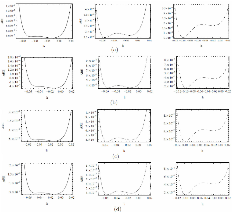
FIGURE 2 Plotting the average residual error for 5-terms of HATM solutions using the Liouville-Caputo, Caputo-Fabrizio-Caputo and Atangana-Baleanu-Caputo operators arranged from left to right with β = 0.7, 0 ≤ ς, ξ ≤ 10, k = 0.001, γ = 0.4, a1 = 0.002, b1 = 0.002, a2 = 0.001, b2 = 0.001.
Figures 1(a)-(d) shows the numerical solutions for ui,ξ (ς, 0), vi,ξ (ς, 0) against h with β = 0.7 k = 0.01, γ = 0.4, ς = 6, ξ = 0, a1 = 0.2, b1 = 0.1, a2 = 1 and b2 = 0.4.
We plot the h-curves of 5-terms of HATM solutions (32)-(33) with the aim to observe the intervals of convergence. In these figures, the straight line that parallels the h-axis provides the valid region of the convergence 30. Now, we compute the optimal values of the convergence-control parameters by the minimum of the averaged residual errors (33-38).
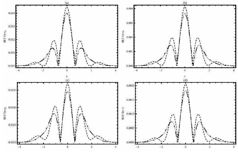
FIGURE 3 Plotting the residual error functions for 4-terms of HATM solutions with β = 0.7, ξ = 20, k = 0.001, γ = 0.4, a1 = 0.002, b1 = 0.002, a2 = 0.001, b2 = 0.001. Solid line (C), Dotted line (CFC), and Dash - Dotted line (ABC).
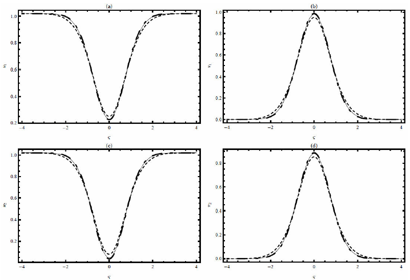
FIGURE 4 The plot of 4-terms of HATM solutions using LC, CFC and ABC operators with β = 0.4, k = 0.01, γ = 0.6, ξ = 15, a1 = 0.8, b1 = 1, a2 = 1, b2 = 0.9. Solid line (C), Dash line (CFC) and Dash-Dot-Dash line (ABC).
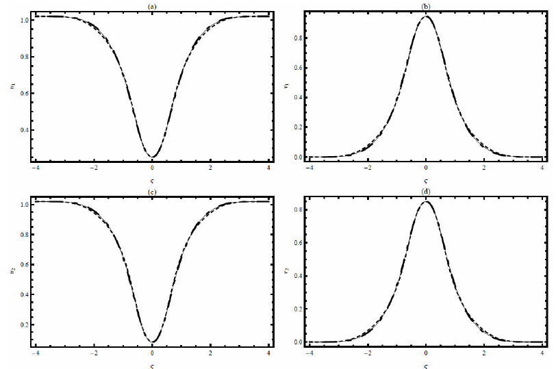
FIGURE 5 The plot of 4-terms of HATM solutions using LC,CFC and ABC operators with β = 0.9, k = 0.01, γ = 0.6, ξ = 15, a1 = 0.8, b1 = 1, a2 = 1, b2 = 0.9. Solid line: (C), Dash line: (CFC), and Dash-Dot-Dash line:(ABC).
corresponding to a nonlinear algebraic equations
Figure 2(a)-(d) and Tables I-II show the averaged residual error for the Liouville-Caputo (C), Caputo-Fabrizio- Caputo (CFC), and Atangana-Baleanu-Caputo (ABC) operators. These figures show the Eui (h) and Evi (h) for 4- terms obtained with HATM. Solutions we set into (34) - (35) Ξ = 10 and Υ = 10 with k = 0.001, γ = 0.4, a1 = 0.002, b1 = 0.002, a2 = 0.001 and b2 = 0.001. Using the command “Minimize” of Mathematica we plotting the residual error against h to get the optimal values h. From Fig. 2 and Tables I-II, we observe the average residual error of order 10−6 − 10−7. This observation assures that the HATM solutions for C, CFC and ABC are converging very rapidly. Figure 3(a)-(d) shows the residual errors functions with C, CFC and ABC operators for (14)-(15) at β = 0.7 It can be seen from these figures the order of REF are very small for all operators. Of Course, we can not say which the better?, due to the operators have a different kernel.
Finally we plot the HATM solutions for C, CFC and ABC fractional derivatives for different values of β. Figures 4-5 show the behavior of the new models with C, CFC and ABC operators for β = 0.4, and 0.9. From these figures, we noted that these new operators identical as the fractional order approaches from the integer order.
TABLE I The average residual error for 4-terms of HATM solutions with β = 0.7, 0 ≤ ς, ξ ≤ 10, k = 0.001, γ = 0.4, a1 = 0.002, b1 = 0.002, a2 = 0.001, b2 = 0.001, using the C, CFC and ABC operators, respectively.
| Operators | Optimal value of hu1 | Minimum of Eu1 (h) |
| C | -0.011844 | 1.542 X 10⁻⁶ |
| CFC | - 0.055422 | 1.465 X 10⁻⁶ |
| ABC | - 0.0973563 | 5.431 X 10⁻⁷ |
| Operators | Optimal value of hv1 | Minimum of Ev1 (h) |
| C | -0.011811 | 1.542 X 10⁻⁶ |
| CFC | -0.055427 | 1.466 X 10⁻⁶ |
| ABC | -0.097383 | 5.438 X 10⁻⁷ |
TABLE II The average residual error for 5-terms of HATM solutions with β = 0.7, 0 ≤ ς, ξ ≤ 10, k = 0.001, γ = 0.4, a1 = 0.002, b1 = 0.002, a2 = 0.001, b2 = 0.001, using the C, CFC and ABC operators, respectively.
| Operators | Optimal value of hu1 | Minimum of Eu1 (h) |
| C | -0. 011900 | 3.133 x 10⁻⁷ |
| CFC | - 0. 053997 | 3.486 x 10⁻⁷ |
| ABC | - 0. 096408 | 1.633 x 10⁻⁷ |
| Operators | Optimal value of hv1 | Minimum of Ev1 (h) |
| C | -0. 011807 | 3.834 X 10⁻⁷ |
| CFC | -0. 055014 | 3.592 X 10⁻⁷ |
| ABC | -0. 097085 | 1.432 X 10⁻⁷ |
5.Conclusion
In this paper, HATM was employed analytically to compute the approximate solutions of FCIACS using the Liouville- Caputo, Caputo-Fabrizio-Caputo and Atangana-Baleanu- Caputo fractional derivatives. The interval of the convergence of HATM and optimal value of h were compute. Also the residual error functions were obtained. The order of the average residual error and residual error functions indicate that the approximations that have been calculated by HATM with C, CFC and ABC fractional derivatives to the accuracy and effectiveness of our results.

