Research
Lorentzian surfaces and the curvature of the Schmidt metric
Y. Sanchez Sanchez1
C. Merlin2
R. Reynoso Fuentes3
1Mathematical Sciences and STAG Research Centre, University of Southampton, United Kingdom Southampton, SO17 1BJ. e-mail: Y.SanchezSanchez@soton.ac.uk
2Centro Brasileiro de Pesquisas Físicas (CBPF), Rio de Janeiro, CEP 22290-180, Brazil. e-mail: cmerlin@cbpf.br
3Departamento de Física, Facultad de Ciencias, Universidad Nacional Autónoma de México (UNAM), Ciudad de México, México. e-mail: rreynoso.92@ciencias.unam.mx
Abstract
The b-boundary is a mathematical tool used to attach a topological boundary to incomplete Lorentzian manifolds using a Riemaniann metric, called the Schmidt metric, on the frame bundle. In this paper we give the general form of the Schmidt metric in the case of Lorentzian surfaces. Furthermore, we write the Ricci scalar of the Schmidt metric in terms of the Ricci scalar of the Lorentzian manifold and give some examples. Finally, we discuss some applications to general relativity.
Keywords: Gravitational singularities; Lorentzian surfaces; Schmidt metric; general relativity; b-boundary
PACS: 0420DW; 0240HW; 0420CV
1. Introduction
One of the biggest surprises that General Relativity (GR) has given us is that under certain circumstances the theory predicts its own limitations. There are two physical situations where we expect the theory to break down. The first one is the gravitational collapse of certain massive stars when their nuclear fuel is spent. The second one is the far past of the universe when the density and temperature were extreme. In both cases, we expect that the geometry of spacetime will show some pathological behaviour.
The nature of a gravitational singularity is a delicate issue. It might be tempting to define a gravitational singularity following other physical theories (such as electromagnetism) as the location where the relevant physical quantities are undefined. However, in the gravitational case this prescription does not work due to the identification of the spacetime background with the gravitational field. As a result, the concepts of ‘spatial location’ and ‘temporal duration’ have meaning only in the domain where the gravitational field is defined. This represents a problem because the size, place and shape of singularities can not be straightforwardly characterised by any physical measurement.
The first mathematical description of a gravitational singularity comes from Penrose and Hawking seminal theorems. They characterised singularities as obstructions to geodesic completeness and managed to show that this happens under certain conditions1. Broadly speaking, the theorems establish that a spacetime (M,g) that satisfies simultaneously:
a condition on the curvature,
an appropriate initial or boundary condition,
and a global causal condition,
must be geodesically incomplete2.
One would like to attach a boundary to the incomplete spacetime to understand the singularity better. The procedure to attach a boundary to a Lorentzian manifold can be done in several nonequivalent ways. In this work we will focus on the b-boundary method3. This method allows a classification of singularities in terms of parallel propagated frames, it distinguishes between points at infinity and points at a finite distance, and it generalizes the idea of affine length to all curves regardless of them being geodesic or not. Other common techniques to attach boundaries to Lorentzian manifolds are conformal boundaries1,4 and the causal boundaries1,5 which we describe below. In addition, we would like to mention other constructions such as the a-boundary6,7 and boundaries constructed from light rays8.
The conformal boundary allows us to study the structure of the metric at “infinity”. The idea of conformal compactification is to bring points at “infinity” on a non-compact pseudo-Riemannian manifold (M,g) to a finite distance (in a new metric) by a conformal rescaling of the metric g̃=Ω2g. This precise definition of conformal compactification only applies to an asymptotically simple spacetime. (M,g) is asymptotically simple, if there are another smooth Lorentz manifold and associated metric (M̃,g̃) such that:
MM̃∂Mthere exists a smooth scalar field Ω on M̃ such that g̃=Ω2g on M, and Ω=0,dΩ≠0 on ∂M;
every null geodesic in M acquires a future and past endpoints on ∂M.
This technique has the evident drawback that it can only be applied to this kind of spacetimes4. Moreover, notice that in Minkowski spacetime the conformal boundary is given by ∂M=I-∪I+ (where I- corresponds to null-past infinity and I+ corresponds to null-future infinity) while io,i+,i- which correspond to spacelike infinity, future timelike infinity, and past timelike infinity respectively do not belong to the conformal boundary (the thorough reader can find in1 formal definitions of I-,I+,io,i+,i-). The reason for this is because ∂M is not a smooth manifold at these points. Despite this, the conformal boundary has been successfully applied to study isolated systems in General Relativity4 and to the AdS-CFT correspondence9,10.
On the other hand, the causal boundary of a spacetime consists on attaching a boundary that depends only on the causal structure. However, this implies on this particular construction that one is not able to distinguish between boundary points and points at infinity. Moreover one has to assume that (M,g) is strongly causal. This construction relies on indecomposable past sets (IP) and indecomposable future sets (IF), which we now define. An open set U is an IP if it satisfies I-(U)⊂U and cannot be expressed as the union of two proper-open subsets V and W, satisfying I-(V)⊂V and I-(W)⊂W respectively. Similarly using I+ one can define IF. The class of IPs can be divided into two classes: proper IPs (PIPs) which are of the form I-(p) for p∈M, and terminal IPs (TIPs) which are not formed by the history of any point in M. We shall denote by M⏞ the set of all IPs of the space (M,g) and M⏟ the set of all IFs of the space (M,g). Originally, one defines a suitable topology on M⏞,M⏟ to identify IFs and IPs and one can form a space M*=M⋃Δ where Δ is called the causal boundary11. However, this topology presents some problems that have led to several redefinitions. A full revision of the causal boundary and its relationship with the conformal boundary can be found in5. Also its relation with boundaries in Riemannian and Fislerian manifolds can be found in11.
There is also the b-boundary. This is a method developed by Schmidt, which allows one to attach a boundary ∂M called the b-boundary to any incomplete spacetime M (or even to any manifold with a connection). The procedure consists on constructing a Riemannian metric for the frame bundle L(M) or the orthonormal bundle O(M), called the Schmidt metric. This metric is then used to generalise the idea of affine length to all curves. This generalisation is important because it helps to unify some elements of Riemannian geometry with Lorentzian geometry. For example, while only in the Riemannian case geodesic completeness implies that every curve is complete; the notion of b-completeness implies completeness of every curve in both signatures. The definition of a curve we are using here is a piecewise-C1 curve.
The structure of this paper is as follows. In Sec. 2 we give a general overview of the mathematical preliminaries needed. In Sec. 3 we describe how the Schmidt metric and the b-boundary are constructed following the procedure by Schmidt 3. In Sec. 4 we discuss the geometry of the orthonormal-bundles for 1+1 conformally flat spacetimes. In the last section, namely Sec. 5, we discuss the results in the context of gravitational singularities in general relativty.
2. Preliminaries
As a first step, let us present some of the required concepts of differential geometry. We present the basic concept of fibre bundles, G-principal bundles, solder forms and connections. The manifolds we consider in this paper are paracompact, C∞, connected, and Hausdorff.
2.1 Fibre Bundles and G-Principal Bundles
A Fibre bundle with fibre F is a manifold E with a surjetive map π:E→M where there is a neighbourhood U at each point p of M such that π-1(U) is isomorphic to U×F, i.e., for each point p∈U there is a diffeomorphism ϕp of π-1(p) onto F such that the map ψ(p¯)=(π(p¯),ϕπ(p¯)) is a diffeomorphism. We call M the base space of the fibre bundle E.
A G-principal bundle P over a manifold M is a fibre bundle where the fibre is a lie group G with a continuous right action Rg that acts freely:
(p¯,g)∈P×G→Rg(p¯)∈Pand satisfies that M is the quotient space of P by the equivalence relation induced by G12.
Let M be a n-dimensional manifold. A frame {Ea}p at point p is an ordered basis of Tp. Let L(M) be the set of all frames {Ea} at all points on M with the projection π sending a frame at p to p. Then the general linear group GL(n,R) has a natural action on {Ea}, i.e., given ({Ea},Aab) the action of Aab∈GL(n,R) on {Ea} is {Eb=AabEa}. If {xa} are coordinates on M and we choose the frame {(∂/∂xa)}, then it can be shown that the coordinates (xa,βba) are a local coordinate system of LM, where βba represent the ab element for the change of basis matrix β between {(∂/∂xa)} and any other frame {Eb}. In fact this choice makes L(M) a G-principal bundle called the frame bundle. Moreover, if we have a metric in M and we restrict the frames to just orthonormal frames, we obtain another G-principal bundle called the orthonormal frame bundle O(M). The associated Lie Group to O(M) is then the orthonormal group, SO(n,R) or SO+(1,n,R). This last definition is signature dependent.
Every tangent space Tp¯P of a G-principal bundle P has a subspace called the vertical subspace Vp¯. This subspace is given by the kernel of the differential Dπ restricted at p¯. Explicitly,
Vp¯={X∈Tp¯P|Dπp¯(X)=0∈Tπ(p)M}.
2.2 Solder form and Connections
The solder form of a frame bundle L(M) is the map:
θ:TL(M)→Rn:Q→p¯-1(Dπ(Q))
where Q is an element of Tp¯LM and p¯ is a linear map from Rn to Tπ(p¯) that sends the canonical vectors to a choice of basis on Tπ(p¯). The solder form for the orthonormal bundle 𝑂(ℳ) is defined similarly. Notice that Vp¯⊂ker(θ).
A connection ∇¯ on a G-principal bundle is an assignment of a subspace Hp¯ called the horizontal subspace of Tp¯(P) for all p¯ in P, such that:
Tp¯P=Hp¯⊕Vp¯Hp¯g=Dp¯Rg(Hp¯)p¯∈Pg∈GA connection form ϖ of a connection ∇¯ in a G-principal bundle is a C∞ map
ϖ:TP→gwith the following properties:
if ϖ(X)=0 then X∈Hp¯ for some p¯ in P,
for all g in G and all C∞ maps X:P→TP
ϖ(DRg(X))=ad*(g-1)ϖ(X), and
for all g⃗∈g,ϖ(Xp¯*)=g⃗ where Xp* is the tangent vector at t=0 of a curve given by γ(t)=Rexptg⃗(p¯).
Let us remind the reader that connections and connection forms uniquely determine one another.
In coordinates, the connection form ϖ is written as ϖ=∑a,bϖbaFba where
ϖ ba=∑c(β-1) cadβb c+∑d,e(β-1) caΓ decβ bedxd,
(1)
where (β-1) ca is the inverse of the matrix β ca and Γ bca are the Christoffel symbols.
The solder form θ is then given by θ=∑aθaea where
θa=∑c(β-1) cadxc,
(2)
and ea is the natural basis of Rn
12.
3. The Schmidt metric
If one thinks of a singularity in classical Newtonian gravity, the statement that the gravitational field is singular at a certain location is unambiguous. As an example, take the gravitational potential of a spherical mass M in Cartesian coordinates
V(t,x,y,z)=GMx2+y2+z2,
where G is the gravitational constant, and the potential exhibits a singularity at the point x=y=z=0, for any time t in R. The location of the singularity is well defined because the coordinates have an intrinsic character which is independent of V.
However, in the case of GR the prescription given above can not work. This is due to the identification of the background spacetime with the gravitational field. Hence, only in the regions where the gravitational field is defined it is meaningful to talk about locations. Consider the spacetime with the line element
ds2=-1t2dt2+dx2+dy2+dz2,
defined on the manifold {(t,x,y,z)∈R∖{0}×R3}. If we say that there is a singularity at the point t=0, we will be speaking too soon for two reasons. The first one is that t=0 is not part of the manifold. It makes no sense to talk about t=0 as a location where the field diverges. The second thing is that the lack of an intrinsic meaning of the coordinates in GR must be taken seriously. By making the coordinate transformation η=log(t), we obtain the line element
ds2=-dη2+dx2+dy2+dz2
on R4, which is an isometric extension of the previously defined spacetime. This spacetime is, of course, Minkowski spacetime which is non-singular .
Another idea is trying to define a singularity in terms of invariant quantities, such as invariant scalars. The reason for this is that if these quantities diverge then it matches our physical idea that objects must suffer stronger and stronger deformations as we encounter the singularity. These scalars are usually constructed from contractions of the Riemann tensor and its derivatives. Unfortunately, these scalars are not well-suited to define the complete geometry. Consider the metric
ds2=dudv+Hij(u)xixjdu2-dxidxi,
given in the coordinates (u,v,x1,x2) and where H(u) is C1. This spacetime is known as a pp-wave spacetime and it can be shown that every polynomial curvature-scalar vanishes, despite the fact that in general the spacetime is not flat13.
A more troublesome feature of using scalars for defining singularities is that they are ‘too local’ in the sense that they are evaluated at given points. Therefore, if the point is removed, the scalar cannot be computed directly and we need an approximation procedure.
A precise mathematical way to approximate the “missing points” is to use convergent sequences of points on the manifold. In this case the formal statement is: “The sequence {R(xn)} diverges while the sequence {xn} converges to y”, where R(xn) is some scalar curvature invariant evaluated at xn in M and y is some point not necessarily in M.
In Riemannian geometry, the notion of distance allows us to define Cauchy sequences {xn} and therefore a notion of convergence. Moreover, if every Cauchy sequence converges in M then every geodesic can be extended indefinitely. This means we can take the domain of every geodesic to be R. In this case, we say that M is geodesically complete. In fact, the converse is also true: if M is geodesically complete then M is metrically complete, i.e., every Cauchy sequence converges to a point in M
14. This allows us to use Cauchy sequences or sequences of points along geodesics as our sequences of points.
The Riemannian case is an useful example, but as soon as we move to Lorentzian geometry, which we take as the correct geometrical setting for GR, the previous discussion cannot be used as stated. The reason is that Lorentzian metrics do not have a distance function defined and, therefore, Cauchy sequences cannot be defined. Thus, one is restricted to the notion of geodesically complete manifolds in the Lorentzian case.
Moreover, the existence of three kinds of vectors available in any Lorentzian metric defines three nonequivalent notions of geodesic completeness -depending on the character of the tangent vector of the curve- spacelike completeness, null completeness and timelike completeness, which are, unfortunately, not equivalent. It is possible to construct spacetimes with the following characteristics15,16,19:
timelike complete, spacelike and null incomplete,
spacelike complete, timelike and null incomplete,
null complete, timelike and spacelike incomplete,
timelike and null complete, spacelike incomplete,
spacelike and null complete, timelike incomplete, or
timelike and spacelike complete, null incomplete.
Furthermore, there are examples of a geodesically null, timelike and spacelike complete spacetimes with an inextendible timelike curve of finite length16,19. A particle following this trajectory will experience bounded acceleration and in a finite amount of proper time its spacetime location would stop being represented as a point in the manifold.
In order to overcome this, Schmidt provided an elegant way to generalise the idea of affine length to all curves, regardless of such curves being geodesic or not. This construction in the case of incomplete curves allows to attach to the spacetime M a topological boundary ∂M called the b-boundary. The procedure for constructing the Schmidt metric consists in building a Riemannian metric in the frame bundle L(M). We use the solder form θ on L(M) and the connection form ϖ on L(M) associated to the Levi-Civita connection ∇ on M to do this. Explicitly, the Schmidt metric is given by
g¯(X,Y)=θ(X)⋅θ(Y)+ϖ(X)∙ϖ(Y)
(3)
where X,Y∈Tp¯P and ⋅,• are the inner products in Rn and g≅Rn2 respectively. The construction of the Schmidt metric is more general and can be applied to any manifold with a connection. This connection does not necessarily need to be a metric compatible connection3. However, as mentioned above, we will use the Levi-Civita connection because we will always assume a metric on the manifold.
Let γ:[a,b]→M be a piecewise C1 curve through p in M. A curve γ¯:[a,b]→L(M) in L(M) is called the lift of the curve γ if it satisfies π(γ¯)=γ and Dπ(γ¯̇)=γ̇. The length of γ¯ with respect to the Schmidt metric is
Lγ¯(b)=∫ab∥γ¯(η)̇∥g¯dη,
which is called the generalised affine-length of γ. We can then use this to re-parametrise γ which generalises the notion of an affine parameter. In the case where 𝛾 is a geodesic parametrised by Lγ(t)¯, it is parametrised with respect to an affine parameter. If every curve in a spacetime M with finite generalised-affine-length has endpoints, we call this spacetime b-complete. If it is not b-complete, we say that the spacetime is b-incomplete.
Notice that if there is a curve γ in M that has finite affine-length and no endpoint, then the lift curve γ¯ cannot have an endpoint. Otherwise, if p¯ is the endpoint of γ¯, π(p¯)=p would be an endpoint of γ contradicting the incompleteness of γ. The previous remark shows that geodesic incompleteness implies b-incompleteness. The converse is not true as Geroch’s example16 shows a b-incomplete spacetime that is geodesically complete. Therefore, b-incompleteness is a generalisation of geodesic incompleteness.
Now given an incomplete spacetime M, using the Riemannian metric g¯ on L(M), we can ‘Cauchy complete’ L(M). Let us denote by L(M)¯ the Cauchy completion of L(M).
We define the quotient space M¯=L(M)¯/G+, where G+ is the connected component of the identity of GL(n;R) under the equivalence of orbits, i.e., (p¯,g)∈L(M)¯∼(q¯,g')∈L(M)¯ if p¯=q¯ and there is h∈GL(n;R) such that g=hg'. This quotient induces a topology in M¯ by taking the finest topology that makes the map π:L(M)¯→M¯ continuous and, therefore M¯ is a topological space. However, it does not imply that M¯ is a manifold. Finally, we can characterise the b-boundary as the set ∂M=M¯∖M.
We repeat the same construction for subgroups of GL(n;R). In particular, a common choice in the Lorentzian case is the subgroup of all Lorentz transformations preserving both orientation and direction of time, which is called the proper orthochronous Lorentz group, and it is denoted by SO+(1,n). In a completely analogous way we can form the quotient M¯=O(M)¯/SO+(1,n;R) and define the b-boundary as the set ∂M=M¯∖M. The completion using SO+(1,n) is homeomorphic to the completion using GL(n;R) . The advantage of this construction is that O(M) is a manifold of dimension n+(n(n-1)/2) instead of the n+n2 dimensions of L(M). Also, the construction can be carried in a manifold with a Riemannian metric, in that case M¯ is homeomorphic to the Cauchy completion of M . This reinforces the conviction that the b-boundary is a natural way to attach boundaries to manifolds with connections.
4. The Schmidt metric of 1+1 spacetimes
In this section, we locally construct the Schmidt metric for general 1+1 spacetimes. Moreover, we find a relationship between the scalar curvature of the Schmidt metric on (O(M), g¯) and the scalar curvature of (M, g). Finally, we give several explicit examples.
Notation: We use overlines to denote the Riemannian geometric quantities that belongs to O(M) while the geometric quantities without any overline belong to the Lorentzian manifold M.
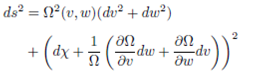
4.1 The Schmidt metric for 1+1 conformal spacetimes
Let M be a 2-D manifold with a Lorentzian metric g and an orthonormal bundle O(M). Then, we can find coordinates (v,w) which locally transform the line element of the metric g to the following form20:
ds2=Ω2(v,w)(-dv2+dw2).
(4)
An orthonormal basis is then given by the vector fields
E1=1Ω∂∂vandE2=1Ω∂∂w.
(5),(6)
The orthonormal basis prescribed above is not unique. Any other orthonormal basis is of the form
Ẽ1=coshχ1Ω∂∂v+sinhχ1Ω∂∂wẼ2=coshχ1Ω∂∂w+sinhχ1Ω∂∂v
(7),(8)
for some χ∈R.
Let us notice that the coefficients of such a basis with respect to (∂/∂v,∂/∂w) define an unique non-singular matrix β with inverse β-1:
β=1Ω(coshχsinhχsinhχcoshχ),andβ-1=Ω(coshχ-sinhχ-sinhχcoshχ).
(9)
These matrices are important in the sense that they are useful to define local coordinates on O(M) as follows:
{v,w,1Ωcoshχ∂∂v+sinhχ∂∂w,1Ωcoshχ∂∂w+sinhχ∂∂v|(v,w)∈M,χ∈R}.
(10)
As stated in Sec. 3, the Schmidt metric g¯ for any X,Y∈TO(M) on O(M) is given by
g¯(X,Y):ϖ(X)⋅ϖ(Y)+θ(X)⋅θ(Y)
(11)
where ϖ is the connection form on O(M) and θ the solder form.
Now let us consider a curve γ¯(s) in O(M) given by γ¯:s∈[a,b]↦(v(s),w(s),β ca(s)) and evaluate θ(γ¯̇) and ϖ(γ¯̇). Explicitly we have
θ(γ¯̇)=Ωv̇coshχ-ẇsinhχ-v̇sinhχ+ẇcoshχ,
(12)
and
ϖ(γ¯̇)=0χ̇+1Ω((∂vΩ)ẇ+(∂wΩ)v̇)χ̇+1Ω((∂vΩ)ẇ+(∂wΩ)v̇)0,
(13)
where we have used [1] and [2]. Then, the line element for the Schmidt metric using a general inner product can be written as:
ds2=Ω2(v,w[(a11cosh2χ+a22sinh2χ)dv2-2(a11+a22)sinhχcoshχdvdw+(a22cosh2χ+a11sinh2χ)dw2+2a12(cosh2χdvdw-sinh2χ(dv2+dw2))]+(b22+2b24+b44)dχ+1Ω∂Ω∂vdw+∂Ω∂wdv2.
(14)
where A=(aij),B=(bij) are symmetric matrixes with positive eigenvalues.
It can be shown that using two different inner products produce two unifomly equivalent metrics18.
In application it is commonly used the Euclidean innner product which give the line element for the Schmidt:
ds2=Ω2(v,w)(cosh(2χ)(dv2+dw2)-2sinh(2χ)dvdw)+dχ+1Ω∂Ω∂vdw+∂Ω∂wdv2.
(15)
We avoid quoting long tensorial expressions for the curvature tensors and give only the result for the Ricci scalar of (15) in terms of Ω and its derivatives, but we have that R¯ is given by
R¯=-12Ω8Ωww-ΩvvΩ-Ωw2-Ωv22-2.
(16)
Taking into account that
R=-2Ω4((Ωww-Ωvv)Ω-(Ωw2-Ωv2))
(17)
This means that Eq. (16) becomes
R¯=-18R2-2
(18)
Notice that in (18) is the relationship between both scalar curvatures. As direct consequence, we can establish the negativity of the Ricci scalar for any Schmidt metric in the Lorentzian signature. In Sec. 5 we give counterexamples that such a condition does not hold in the Riemannian case. Also, Eq. (18) has been obtained using the Levi-Civita connection. Therefore, using another connection, even in the Lorentzian case, may not hold.
Now we calculate such scalar curvatures for some physical spacetimes.
4.2 The Schmidt metric of Minkowski spacetime
We can write the Schmidt metric in the form
ds2=(dt2+dx2)cosh(2χ)-2dtdxsinh(2χ)+dχ2.
(19)
Now let us consider the change of coordinates: t=u+ṽ,x=u-ṽ and write:
ds2=2(cosh2χ+sinh2χ)du2+2(cosh2χ-sinh2χ)dv~2+dχ2
(20)
or in an equivalent manner
ds2=2e2χdu2+2e-2χdṽ2+dχ2.
(21)
We explicitly calculate R¯ab and get
R¯χχ=-2,
(22)
and all other components are zero. The Ricci scalar is then
R¯=-2.
(23)
Hence, the geometry in the bundle is not flat even if Minkowski spacetime is flat.
4.3 The Schmidt metric of Friedmann-Robertson-Walker (FRW) spacetime
For simplicity, let us consider the case of the 1+1 FRW cosmological model which can be obtained from the 4-dimensional one by collapsing two spatial coordinates. This is equivalent to considering the injection map
h:(η,x)→(η,x,y0,z0):M→N=M×Σ,
(24)
where Σ is a suitable two dimensional manifold. This way the four dimensional metric reduces to
ds2=ηq(-dη2+dx2),
(25)
for any value of q>0. The Ricci scalar corresponding to the spacetime described by (25) is
R=-qη-2-q.
(26)
From Eq. the Schmidt metric in O(M), for our case study, takes the form
ds2=ηq(cosh(2χ)(dη2+dx2)-2sinh(2χ)dηdx)+(dχ+qηdx)2.
(27)
Using computer algebra we calculated the Ricci tensor for the line element . In components it is given by
And the Ricci scalar is
R¯=-2-18q2η-2(2+q),
(28)
which can equivalently be obtained from Eq.(18).
4.4 The Schmidt metric of De Sitter and Anti-De Sitter spacetimes
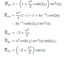
Let us now consider the De Sitter and Anti-De Sitter models and study the behaviour of the corresponding curvature scalars. First, consider the De Sitter case. The two dimensional De Sitter spacetime for closed spatial sections is defined with the line element
ds2=-dτ2+α-2cosh2(ατ)dω2.
To obtain the conformal form we make the change tan(η/2)=tanh(ατ/2), which leads to
ds2=1α2cos2(η)(-dη2+dω2).
(29)
In these coordinates (η,ω) De Sitter space is conformal to the static Einstein universe1. The Ricci scalar for is then
R=2α2.
(30)
Using Eq.(15) we get
The Ricci tensor is computed by taking Ω=1/αcos(η). The non-vanishing components are:
Thus the Ricci scalar is
R¯=-2-α42.
Notice that in the limit as α→0 we recover the Minkowski limit once again.
Now let us look at the Anti-De Sitter spacetime. The two dimensional Anti-De Sitter metric has the line element
ds2=1α2y2(-dt2+dy2)with y>0. The Ricci scalar is
R=-2α2.
(32)
We identify Ω=1/αy and using Eq.(15) we obtain
Where the non-vanishing components of the Ricci tensor are
R¯tt=-2+α4-α2cosh(2χ)2y2,R¯yy=-2+α2cosh(2χ)2y2,R¯χχ=-2+α42,R¯ty=α2cosh(χ)sinh(χ)y2,R¯tχ=--4+α42y,
and its trace is given by
R¯=-2-α42.
Notice that for spacetimes that behave asymptotically as Anti-De Sitter spacetime, the curvature would behave similarly as in the Anti-De Sitter case as one approaches the asymptotic region. Moreover, in many applications such as in the AdS/CFT correspondance one uses a conformal compactification. In those cases it is neccesary to compute the curvature again because the curvature is not a conformal invariant.
5. Discussion
In our exposition, we obtained Eq.(15) which is the line element of the Schmidt metric for all 1+1 Lorentzian manifolds M. This line element determines, via the curvature, all the local isometric invariants. If ∂M=∅, then the 3-manifold corresponds to the orthonormal bundle where the fibres of the bundle are SO+(1,1)≅R. Therefore, O(M) is not compact. If ∂M≠∅, then the 3-manifold is not necessarily a G-bundle (the group may not act freely or transitively). In fact there are general geometric conditions on the curvature to guarantee that the fibres above a boundary point are degenerate24. This is, for example, the case when M is the Friedmann-Robertson-Walker spacetime. Then O(M)¯ is not a G-bundle as the fibre over the singularity is a point instead of a copy of SO(1,1)+(M). Moreover, if there is a singularity not only in the past but also in the future both singularities are identified as the same boundary point23. The degeneracy of the fibre also affects the topology of M¯, which in the Friedmann-Robertson-Walker case is no longer Hausdorff. In fact this topological behaviour is expected in general spacetimes when the fibre totally degenerates such as in Schwarzschild and Kasner metrics . However, there has been mathematical developments which allow to circumvent this undesirable situation by taking a canonical minimum refinement of the topology in the completion M which T2-separates the spacetime M and its boundary ∂M. Notice that this result does not guarantee that points which one may consider physically different such as the initial and final singularity in a closed Friedmann-Robertson-Walker scenarios are not identified. In order to achieve such separation, certain modifications to the completion process have been suggested23. The b-boundary has also given some results that link the geometry27 of principal bundles with that of the base manifold and with non-commutative geometry26. Moreover, it has been shown that in four dimensions the Friedmann-Robertson-Walker and Schwarzschild b-completion ∂M is a point21,23,28.
The notion of b-incomplete spaces allows us to describe incomplete curves in manifolds with connections. Our initial motivation to study this, was to develop the language to describe pathologies in the geometry as we approach points that in some sense are “boundary points" of the manifold. One can describe how the main manifestation of gravity in GR, the curvature of the manifold, can behave along 𝑏-incomplete curves. This is the scheme proposed by Ellis and Schmidt to classify singularities29,30. In particular, they defined that if p∈∂M and there is some scalar constructed from the tensors gab, R bcda and r-covariant derivatives of R bcda that does not behave in a C0 way, then p is a Cr scalar singularity. Using this definition we have the following result
Theorem 1. Let γ¯s:[0,a]→O(M) be a lift from a curve γt:[0,b]→M such that γ(b)∈∂M. If R¯→-∞ as s→a then |R|→∞ as t→b and γ(b)is a scalar singularity.
The proof follows directly from Eq. [18].
Notice that the hypothesis of this theorem together with the hypothesis of any of the Hawking and Penrose theorems gives a singularity theorem in which it is guaranteed that curvature blow up exist. This is in contrast with the usual singularity theorem in which only geodesic incompleteness can be shown.
The theorem above and the singularity theorems implicitly assume a characterisation of singularities in terms of incomplete curves. This notion of singularity captures the idea that there are ‘obstructions’ within the history of point-like observers. In the future one would like extending those theorems to relate these obstructions to curvature blow-up and ill-possessedness of initial value problems of field equations. This approach constitutes most of the research program on the Strong Cosmic Censorship conjecture31,32, the idea behind generalised hyperbolicity33,34,35,36 and field regularity37,38,39,40,41,42.
Appendix
A. The Riemannian case
As it was mentioned in Sec. 5, in the Riemannian case there are three conformally distinctly connected Riemann surfaces (the disc, the plane and the sphere). Moreover, in this case the fibres in O(M) are SO(n,R) which is a compact group. Below we give the Schmidt metric for the general case of 1+1 Riemannian manifolds and compute the curvature scalar for the disc, the sphere and the hyperbolic plane.
In the Riemannian case it is a well know fact that if M is a 2-D manifold with a Riemannian metric we can find coordinates (v,w) which transform locally the line element of the metric to a conformally flat form. Therefore, we have
ds2=Ω2(v,w)(dv2+dw2).
(A.1)
An orthonormal basis is given by the vector fields
E1=1Ω∂∂v,andE2=1Ω∂∂w.
(A.2),(A.3)
Any other orthonormal basis is constructed as a linear combination of as
for some χ∈R. Let us notice that the coefficients of basis with respect to ∂∂v,∂∂w define a unique matrix β and its inverse β-1:
E~1=cosχ1Ω∂∂v+sinχ1Ω∂∂w,andE~2=cosχ1Ω∂∂w+sinχ1Ω∂∂v
(A.4),(A.5)
Notice the main difference with the Lorentzian case in the definition of the matrix β.
The Schmidt metric g¯ on O(M) is given by
g¯(X,Y):ϖ(X)⋅ϖ(Y)+θ(X)⋅θ(Y),
(A.7)
for X,Y∈TO(M). where
θ(γ̇)=Ωv̇cosχ-ẇsinχv̇sinχ+ẇcosχ
(A.8)
and
ϖ(γ˙)=(0-(χ˙+1Ω((∂vΩ)w˙+(∂wΩ)v˙))χ˙+1Ω((∂vΩ)w˙+(∂wΩ)v˙)0)
(A.9)
giving the line element for the Schmidt metric:
The plane
The euclidean metric on the plane is given by the line element
ds2=dv2+dw2
(A.11)
which is characterised by R=0.
Then using Eq.(A.10) we have that the line element for the corresponding Schmidt metric is
ds2=dv2+dw2+dχ2
(A.12)
which is just the flat metric in O(M) so we have R¯=0 which violates the bound given by Eq.18.
The sphere
The round metric on the sphere is given by the line element
ds2=dθ2+sin2(θ)dφ2.
(A.13)
Eq. (A.13) can be expressed in terms of isothermal coordinates (v,w) as
ds2=1cosh2v(dv2+dw2).
(A.14)
This metric is characterised by R=1.
In a similar manner as we did for the plane metric we use Eq.(A.10) to get the line element for the Schmidt metric:
ds2=1cosh2v(dv2+dw2)+(dχ-tanh(v)dw)2,
(A.15)
with curvature scalar R¯=3/2. Notice that in this case the curvature scalar is positive which for Lorentzian manifolds can not happen as a result of Eq.18.
Acknowledgments
Y.S.S and C.M acknowledge funding support from CONACyT. Y.S.S also acknowledge funding support from the Riemann Fellowship. The authors also thank James Vickers, Didier Solis and Oscar Palmas for comments on previous drafts of the paper.
REFERENCES
1. S. W. Hawking and G. F. R. Ellis, The Large Scale Structure of Space-Time. 1st Edition, (Cambridge University Press, 1973).
[ Links ]
2. J. M. M. Senovilla, .. General Relativity and Gravitation 30 (1998) 701-848.
[ Links ]
3. B. G. Schmidt, .. General Relativity and Gravitation 1 (1971) 269-280.
[ Links ]
4. J. Frauendiener, .. Living Reviews in Relativity 7 (2004) 1.
[ Links ]
5. J. L. Flores, J. Herrera and M. Sánchez, .. Advances in Theoretical and Mathematical Physics 15 (2011) 991-1057.
[ Links ]
6. S. M. Scott and P. Szekeres, .. Journal of Geometry and Physics 13 (1994) 223-253.
[ Links ]
7. B. E. Whale, M. J. S. L. Ashley and S. M. Scott, .. Classical and Quantum Gravity 32 (2015) 135001.
[ Links ]
8. R. J. Low, ”The Space of Null Geodesics (and a New Causal Boundary)?? in Analytical and Numerical Approaches to Mathematical Relativity (Springer Berlin Heidelberg, 2006), pp.35-50.
[ Links ]
9. E. Witten, .. Advances in Theoretical and Mathematical Physics 2 (1998) 253-291.
[ Links ]
10. D. Marolf and S. F. Ross, .. Classical and Quantum Gravity 20 (2003) 4085.
[ Links ]
11. J. L. Flores, J. Herrera and M. Sánchez, .. Memoirs of the American Mathematical Society. 226 (2013) No.1064.
[ Links ]
12. S. Kobayashi and K. Nomizu, Foundations of Differential Geometry (Wiley, 1996).
[ Links ]
13. G. W. Gibbons, .. Communications in Mathematical Physics 45 (1975) 191-202.
[ Links ]
14. M. do Carmo, Riemannian Geometry. Birkhäuser, 1992.
[ Links ]
15. W. Kundt, .. Zeitschrift fur Physik 172 (1963) 488-489.
[ Links ]
16. R. Geroch, .. Annals of Physics 48 (1968) 526-540.
[ Links ]
17. A. M. Amores and M. Gutierrez, .. Nonlinear Analysis: Theory, Methods & Applications 47 (2001) 2959-2970.
[ Links ]
18. C. T. J. Dodson, .. International Journal of Theoretical Physics 17 (1978) 389-504.
[ Links ]
19. J. K. Beem, .. General Relativity and Gravitation 7 (1976) 501-509.
[ Links ]
20. T. Weinstein, An Introduction to Lorentz Surfaces (De Gruyter, 1996).
[ Links ]
21. B. Bosshard, .. Communications in Mathematical Physics 46 (1976) 263-268.
[ Links ]
22. R. A. Johnson, .. Journal of Mathematical Physics 18 (1977) 898-902.
[ Links ]
23. C. T. J. Dodson. .. International Journal of Theoretical Physics. 17 (1978) 389-504.
[ Links ]
24. F. Ståhl, .. Communications in Mathematical Physics, 208 (1999) 331-353.
[ Links ]
25. J.L. Flores, J. Herrera and M. Sánchez, .. Journal of Mathematical Physics. 57 (2016) 022503.
[ Links ]
26. F. Ståhl, The Geometry of the Frame Bundle over Spacetime, ArXiv:0006049. (2000).
[ Links ]
27. M. Heller, Z. Odrzygozdz, L. Pysiak and W. Sasin, .. Journal of Mathematical Physics 48 (2007) 092504.
[ Links ]
28. A. M. Amores and M. Gutierrez, .. Journal of Geometry Physics 29 (1999) 177-197.
[ Links ]
29. G. F. R. Ellis and B. G. Schmidt, .. General Relativity and Gravitation 10 (1979) 989-997.
[ Links ]
30. G. F. R. Ellis and B. G. Schmidt, .. General Relativity and Gravitation 8 (1977) 915-953.
[ Links ]
31. M. Dafermos, .. Communications on Pure and Applied Mathematics 58 (2005) 445-504.
[ Links ]
32. Y. Choquet-Bruhat, General Relativity and the Einstein Equations 1st Edition, OUP Oxford, 2009.
[ Links ]
33. C. J. S. Clarke, .. Classical and Quantum Gravity 15 (1998) 975.
[ Links ]
34. J. A. Vickers and J. P. Wilson, Generalised hyperbolicity: hypersurface singularities, ArXiv:0101018.
[ Links ]
35. Y. Sanchez Sanchez and J. A. Vickers, .. Journal of Mathematical Physics 58 (2017) 022502.
[ Links ]
36. Y. Sanchez Sanchez and J.A. Vickers, .. Classical and Quantum Gravity 33 (2016) 205002.
[ Links ]
37. R. M. Wald, .. Journal of Mathematical Physics. 21 (1980) 2802-2805.
[ Links ]
38. B. S. Kay and U. M. Studer, .. Communications in Mathematical Physics 139 (1991) 103-139.
[ Links ]
39. G. T. Horowitz and D. Marolf, .. Physical Review D. 52 (1995) 5670-5675.
[ Links ]
40. A. Ishibashi and A. Hosoya, .. Physical Review D. 60 (1999) 104028.
[ Links ]
41. J. P. Wilson, .. Classical and Quantum Gravity. 17 (2000) 3199-3209.
[ Links ]
42. Y. Sanchez Sanchez, .. General Relativity and Gravitation. 47 (2015) 80.
[ Links ]


 nueva página del texto (beta)
 Inglés (pdf)
 Artículo en XML
 Referencias del artículo
 Enviar artículo por email
 Citado por SciELO
  Similares en
SciELO
Similares en
SciELO 
 Permalink
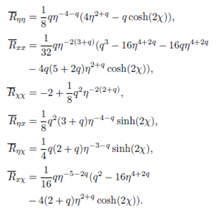
 (31)
(31)

 (A.10)

