


 nova página do texto(beta)
 Inglês (pdf)
 Artigo em XML
 Referências do artigo
 Enviar este artigo por email
 Citado por SciELO
  Similares em
SciELO
Similares em
SciELO 
 Permalink
1. Introduction
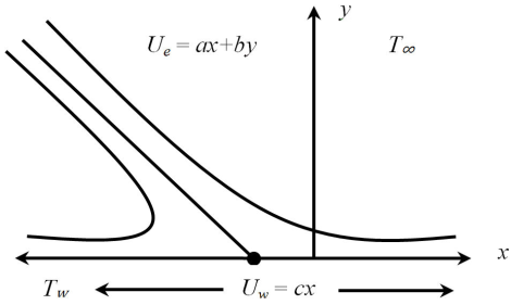
A stagnation-point arises when fluid strikes at a surface and, its velocity becomes zero. During the last few decades, stagnation point flows have been studied by many researchers. The interest of researchers in stagnation point flow is due to its wide applications in industrial and engineering problems, such as cooling of nuclear reactors and electronic devices by fans, solar central receivers exposed to wind currents 1-3, the environment 4 and several others. The maximum heat transfer and pressure gradient are observed in the region of the stagnation point flow. Figure 1 shows that the fluid strikes at a stretching surface with an arbitrary angle of incidence, and the fluid away from the surface moves with the free stream velocity
Unlike Newtonian fluid model, which are governed by a single constitutive equation, non-Newtonian fluid models are complex and it is hard to express them in a single constitutive equation. Different types of models have been proposed by many researchers due to their applications in industries. Amongst these models, the Maxwell model has received a special attention due to its simplicity describing the rheological effects of viscoelastic fluids. Wang and Tan 3, used modified Maxwell model to study the linear stability with soret effects. They found that oscillatory convection of system destabilized by the soret effect and instability of the system increases with the increase of relaxation time. Noor Fadiya 14 studied the hydromagnetic flow of Maxwell fluid under thermophoretic effects and found Homotopic solutions and analyzed that the boundary layer thickness is decreasing function of thermophoretic parameter. Javed and Ghaffari 5, generalized the idea of stagnation point flow of Maxwell fluid. Abel et al. 16, Mukhopadhyay 17, Nadeem et al. 18 also carried out further studies.
Flow over a stretching surface has significant importance due to its extensive use in industries such as wire drawing, hot rolling, cooling of metallic sheets, glass fibers, and many others. Magyari and Keller 19 widely discussed this topictheoretically and numerically. During the last few decades, the study of stagnation point flow over a stretching surface has remained an interesting problem for many researchers. Crane 20 was the first, who studied the stretching sheet problem and found analytical solution. Rajagopal et al. 21 was among the earlier scientists who studied the flow of a viscoelastic fluid over a stretching sheet, Mahapatra and Gupta 22 discussed magnetic effects in the region of the stagnation point flow over a stretching sheet. Nazar et al. 23 investigated a micropolar fluid flow over a stretching sheet in the stagnation point region. Later, Layek et al. 24 Hayat et al. 25, Zhu et al. 26, and Bhattacharyya 27 discussed various effects of the stagnation point flow on linear and non-linear stretching surface.
During the technological processes at high temperatures (e.g. cooling glass sheet etc.), thermal radiation effects play an important role which cannot be neglected. Gupta and Gupta 28 studied the heat transfer over a stretching surface with suction or blowing and discussed the different aspects of the problem. Recently, Mahapatra and Gupta 29 investigated heat transfer in stagnation point region toward a stretching sheet. Raptis et al. 30 studied the effects of thermal radiation on hydromagnetic flow. Pop et al. 31 extended the work of Mahapatra and Gupta by introducing radiation effects. In present problem study of oblique stagnation point flow of Maxwell fluid with radiation effects over a stretching sheet has been carried out numerically using parallel shooting technique. Effects of different parameter on heat and fluid flow are discussed through tables and graphs. in detail. An excellent agreement of results has been found with Pop et al. 31 and Labropulu et al. 32.
2. Flow equations
In present study, steady two-dimensional oblique stagnation point flow of Maxwell fluid over a stretching sheet is considered. The stretching sheet is taken along the plane
Where “div” represents divergence operator,
where
where
The operator
Applying divergence on both sides of Eq. (5), we get
operating
The second factor on left side of the above equation is a vector, using Eqs. (7) and (1), Eq. (10) takes the following form in components
 (11)
(11)
 (12)
(12)
The boundary conditions of the current flow problem are 29
where a, b and c are positive constants having dimension (time)-1. By using boundary layer approximation 31, the above equations reduce to the following form
 (14)
(14)
Introducing the following transformation as suggested by Labropulu et al.29
We obtain the following equation in dimensionless form
 (16)
(16)
and boundary conditions take the form as
Let us assume that ambient temperature of the fluid is
 (18)
(18)
and boundary conditions are
where Pr is the Prandtl number,
By using the continuity equation, we define the stream function
Now substituting Eq. (21) in Eqs. (16-19)
 (22),(23),(24)
where
where the functions
 (26),(27)
After eliminating the pressure, Eq. (26) takes the form as
 (29)
(29)
where A is a constant that accounts the boundary layer displacement. After comparing the coefficients of x 1 and x 0 in Eq. (29), following system of equations is obtained
Energy equation is
and boundary conditions are
Where the prime denotes the derivative with respect to y. For the simplicity, a new variable is introduced which is defined as
It is necessary to mentioned here that for a Newtonian fluid (
The physical quantity of interest is the local Nusselt number, which is defined as
Upon using dimensionless variables given in Eq. (15) the above equation reduces to
3. Numerical method
Non-linear equations (30), (32), and (34) subject to the boundary conditions (33) and (35) have been solved numerically by using parallel shooting method 34. For the solution of highly non-linear problems, the parallel shooting method is better as compared to the simple shooting method because the simple shooting method is hard to use due to its dependence on initial guess. The method of parallel shooting is very efficient for the solution of this kind of problems. The method is described as follows
Equations (30), (32) and (34), are reduced in the system of first order differential equations by letting
and boundary conditions are expressed as
The domain [
The problem is solved over each subinterval such that it satisfies the boundary conditions at
Initial guess is supplied for the first interval and then the obtained solution is taken as initial guess for the next interval and so on.
Algorithm is developed in MATLAB R2010a.
4. Results and discussion
The nonlinear ordinary differential Eqs. (30), (32), and (34) with boundary conditions (33) and (35) have been solved numerically. The numerical values of f″(0), ℎ′(0), A and Nusselt number are shown in tables. In Table I, the comparison is given for
Table I The Numerical values of f''(0), h'(0) and A for the different values a/c, for Newtonian fluid (ß = 0).
| a/c | f''(0) Ref. 31 | present | h''(0) Ref. 31 | present | A Ref. 31 | present |
| 0.1 | -0.96938 | -0.96939 | 0.26278 | 0.26338 | 0.79170 | 0.79170 |
| 0.3 | -0.84942 | -0.84942 | 0.60573 | 0.60633 | 0.51949 | 0.51950 |
| 0.8 | -0.29938 | -0.29939 | 0.93430 | 0.93473 | 0.11452 | 0.11453 |
| 1 | 0.0 | 1 | 1 | 0 | 0 | |
| 2 | 2.01750 | 2.01749 | 1.16489 | 1.16521 | -0.41040 | -0.41041 |
| 3 | 4.72928 | 4.72924 | 1.23438 | 1.23464 | -0.69305 | -0.69305 |
| 4 | 8.00042 | 8.00036 | 1.27272 | 1.27300 | -0.91650 | -0.91650 |
the Table I that the value of 𝑓″(0) is increasing with the increase of 𝑎/𝑐. The comparison of Nusselt number with the result obtained by Pop et al. 31 is shown in Table II. The results shown in braces are reported by Pop et al. 31. Present results as a limiting case are shown in the Tables I and II, which establish a good agreement with the previous results. However, a small difference arises due to change in numerical technique. In present study the parallel shooting method is used where Pop et al. 31 solved with thehelp of simple shooting method. For infinite domain, simple
Table II The Numerical values of Nusselt number for the different values of ß, a/c and Pr.
| Newtonian fluid (ß = 0) | Maxwell fluid (ß = 0:2) | ||||||||
| a/c | Pr | θw=1.1 Rd=1 | Rd=10 | θw=2 Rd=1 | Rd=10 | θw=1.1 Rd=1 | Rd=10 | θw=2 Rd=1 | Rd=10 |
| 0.1 | 0.05 | 0.11617 (0.1159) | 0.25815 (0.2587) | 0.17507 (0.1750) | 0.47034 (0.4737) | 0.11395 | 0.25587 | 0.17287 | 0.46827 |
| 0.5 | 0.52056 (0.5194) | 0.98655 (0.9861) | 0.72129 (0.7210) | 1.64850 (1.6473) | 0.50358 | 0.96460 | 0.69977 | 1.62669 | |
| 1.0 | 0.83618 (0.8337) | 1.53603 (1.5335) | 1.15670 (1.1550) | 2.47460 (2.4763) | 0.81017 | 1.49404 | 1.11685 | 2.43044 | |
| 1.5 | 1.09838 (1.0946) | 2.00807 (2.0040) | 1.53495 (1.5318) | 3.16612 (3.1654) | 1.06728 | 1.94792 | 1.48047 | 3.09981 | |
| 0.05 | 0.21346 (0.2131) | 0.53127 (0.5305) | 0.34720 (0.3465) | 1.00664 (1.0013) | 0.21240 | 0.53059 | 0.34608 | 1.00489 | |
| 0.5 | 0.5 | 0.72884 (0.7267) | 1.74413 (1.7461) | 1.15842 (1.1573) | 3.246117 (3.2408) | 0.72128 | 1.73363 | 1.14868 | 3.23508 |
| 1.0 | 1.06582 (1.0621) | 2.51678 (2.5121) | 1.68455 (1.6823) | 4.64451 (4.6404) | 1.05397 | 2.49782 | 1.66709 | 4.62336 | |
| 1.5 | 1.33262 (1.3268) | 3.12665 (3.1194) | 2.10291 (2.0988) | 5.73795 (5.7386) | 1.31792 | 3.09850 | 2.07912 | 5.70632 | |
| 0.05 | 0.28805 (0.2888) | 0.73736 (0.7517) | 0.47746 (0.4772) | 1.40927 (1.4104) | 0.28805 | 0.73736 | 0.47746 | 1.40927 | |
| 0.5 | 0.91092 (0.9081) | 2.33066 (2.3283) | 1.50985 (1.5085) | 4.45631 (4.4574) | 0.91092 | 2.33066 | 1.50985 | 4.45631 (4.4574) | |
| 1.0 | 1.0 | 1.28824 (1.2833) | 3.29605 (3.2882) | 2.13525 (2.1315) | 6.30218 (6.2985) | 1.28824 | 3.29605 | 2.13525 | 6.30218 |
| 1.5 | 1.57778 (1.5699) | 4.03682 (4.0268) | 2.61515 (2.6098) | 7.71856 (7.7089) | 1.57778 | 4.03682 | 2.61515 | 7.71856 | |
| 0.05 | 0.39551 (0.3948) | 1.02982 (1.0292) | 0.66345 (0.6627) | 1.98097 (1.9811) | 0.39506 | 1.01129 | 0.65865 | 1.90525 | |
| 0.5 | 1.18876 (1.1842) | 3.17994 (3.1738) | 2.02722 (2.0242) | 6.18570 (6.1801) | 1.20143 | 3.18483 | 2.04074 | 6.14863 | |
| 2.0 | 1.0 | 1.64141 (1.6332) | 4.43873 (4.4280) | 2.81466 (2.8093) | 8.68359 (8.6779) | 1.66308 | 4.46166 | 2.84334 | 8.67191 |
| 1.5 | 1.97902 (1.9675) | 5.38551 (5.3690) | 3.39844 (3.3938) | 10.57659 (10.5729) | 2.00662 | 5.42352 | 3.44386 | 10.58412 | |
shooting method is hard to use due to its dependence on initial guess. In present study, the boundary edge reaches to
The effects of parameters namely, the velocity ratio parameter a/c, the Deborah number
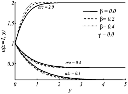
Figure 2 Variation in horizontal velocity profile u along y for the different values of ß, when a/c = 0:1, 0.4, 2.0 and ɤ = 0.
Figure 3 illustrates that the velocity in the case of non-orthogonal stagnation point flowis greater than that of orthogonal stagnation point flow. Figures 4 and 5 show the temperature profiles for the different values of the radiation-conduction parameter Rd and surface heating parameter respectively. In both figures, the thermal boundary layer thickness increases with the increase of radiation-conduction parameter and surface heating parameter. Figure 6 shows the effects of Prandtl number on the temperature profile for small and large values of a/c. It depicts that with the increase of Prandtl number, the thermal boundary layer thickness decreases, meaning that fluids of high Prandtl number are responsible for more heat transfer. The effects of Deborah number ß on temperature profile have also been shown in Fig. 7(a,b) for both small and large values of Prandtl number. Figure 7(a) shows the temperature profile for
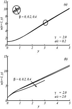
Figure 3 Variation in horizontal velocity profile u along y, for the different values of ß, when (a) a/c = 0:2, (b) a/c = 2:0 and ɤ = 2:0 are fixed.
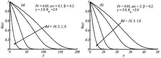
Figure 4 Variation in temperature profile µ(y) for the different values of Rd, when Pr = 0.05, ß = 0:2, ɤ = 5:0, and θw = 2:0 are fixed.
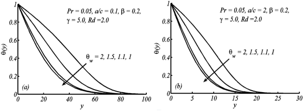
Figure 5 Variation in temperature profile θ(y) for the different values of θw, when Pr = 0.05, ß = 0:2, ɤ = 5:0, and Rd= 2:0 are fixed.
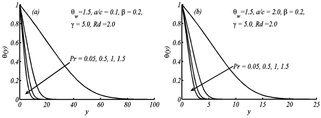
Figure 6 Variation in temperature profile θ(y) for the different values of Pr, when θw = 1:5, ß = 0:2, ɤ = 5:0, and Rd= 2:0 are fixed.
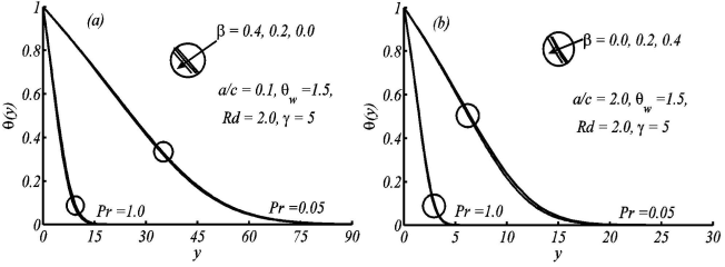
Figure 7 Variation in temperature profile θ(y) for the different values of a/c, when Pr = 0.05, ß = 0:2, ɤ = 5:0, and θw = Rd = 2:0 are fixed.
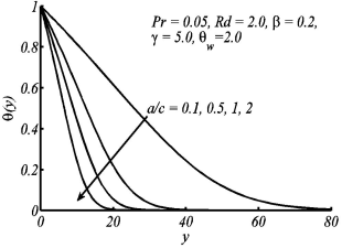
Figure 8 Variation in temperature profile θ(y) for the different values of a/c, when Pr = 0.05, ß = 0:2, ɤ = 5:0, and θw = Rd = 2:0 are fixed.
Figures 9 and 10 show the flow pattern of the oblique stagnation point flows (𝛾≠0). Both cases of favorable (
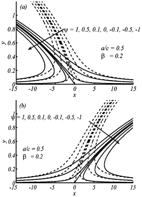
Figure 9 Streamlines for oblique flow (a) ɤ= 10(dashedlines), ɤ = 30(solidlines) (b) ɤ = -10(dashedlines) ɤ = -30(solidlines). when ß = 0:2, a/c = 0:5 are fixed.
Concluding remarks
The radiation effects on the flow of Maxwell fluid near the oblique stagnation point over a stretching sheet is studied. The effects of different parameters on heat and fluid flow are discussed through graphs and tables. This study concludes that the boundary layer thickness decreases with increase of a/c in the oblique stagnation point flow. The thermal boundary layer thickness increases with the increase of radiation-conduction and surface heating parameters. It is also noted that with the increase of free stream velocity the temperature of the fluid decreases near the wall. On the other hand, temperature of the fluid increases with increase of stretching velocity. The velocity of the fluid also increases with the increase of shearing parameter 𝛾.

