1. Introduction

The determination of the polarimetric linear response to light is an important procedure related with the characterization of materials that can be employed in optics and photonics applications. The determination of the Mueller matrix through the Stokes vectors, in principle, provides all the basic information related with the response to any incident polarization state ^1,2. The Mueller matrix can be determined by using different techniques, such as the Ideal Polarimetric Arrangement (IPA), which is based on the linear, ideal response of the polarization components ^1-4. IPA considers the incidence and analysis of at least 4 conventional polarization states, for a total of 16 intensity measurements. A polarization state with both spatially homogeneous amplitude and phase electric field distribution is known as a conventional polarization.

On the other hand, the generation, detection, and application of spatially non-homogeneous polarization states, or unconventional polarization, has generated an increasing interest lately ^5-8. There are some unconventional polarization modes or states, which can not be described as a single product of spatial distribution and polarization states; that is, they show an entangled behavior between their two degrees of freedom. In this sense, the radial and the azimuthal unconventional polarizations are being considered as classically entangled polarization states ^8-12. The use of a single incident classical entangled polarization state (radial polarization) has been considered for the determination of the Mueller matrix (MM) associated to transparent birefringent samples in metrology applications ¹³. Even though this proposal is theoretical, authors have put forward a complex experimental setup to get the MM in a single shot ¹³.

In the work reported here, inspired by Ref. ¹³, we propose, and experimentally demonstrate, a modified configuration to obtain the MM associated to transparent, nondepolarizing systems, using an azimuthally polarized state as the single incident classically entangled polarization state. We have substituted the photodetectors proposed in Ref. 13 by a single CMOS camera, and we have used only one modified Mach-Zehnder interferometer, MMZI, but in essence, we have followed all the remaining suggestions. We have employed the open space and a half- and a quarter-wave plates as the systems under study.

2. Theory

The linear response of a medium to light can be expressed in terms of the Mueller and the Stokes formulism as:

where Si,o represent the incident and the outgoing 4 x 1 Stokes vectors, and M is the 4 X 4 MM of the system under study. A Stokes vector is the algebraic representation of any polarized state, in terms of intensities; for example, the Stokes vector associated to a monochromatic plane wave propagating along the z-direction, with respect to a Cartesian coordinate system, is given by:

where (Ex,Ey) are the orthogonal components of the electric field, * is the complex conjugate operator, and Ip is the intensity associated to the polarizations linear horizontal (x), linear vertical (y), linear diagonal at +45∘, linear diagonal at -45∘, circular right-hand (r) and circular left-hand (l). The azimuthal polarization, Eϕ, can be expressed in terms of different basis sets of spatial modes and polarization distributions, which can be written as (according to the notation employed in ¹³):

where ψ±=(ψ10±ψ01)/2, e^±=(e^x±e^y)/2, ψL=(ψ10+iψ01)/2, ψR=(ψ10-iψ01)/2, e^L=(e^x+ie^y)/2, e^R=(e^x-ie^y)/2, ψ10, ψ01, represent the Hermite-Gauss solution of the paraxial wave equation of order N=m+n ¹³, and e^x, e^y and e^z are the unitary vectors associated to a Cartesian coordinate system.

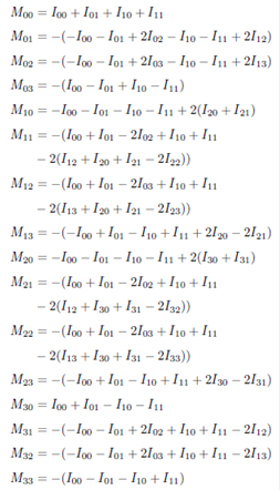
The expressions that relate the intensity measurements to the elements of the MM, for the case of azimuthal polarization as the probe beam, were derived following the formalism presented in Ref. ¹³, resulting in:

(4)

We must remark that the matrix M, obtained through expressions (4), was later transformed to the corresponding MM in the optical convention, MBW through ¹⁴:

where MBW is the MM as defined by Born and Wolf (optical convention), QBW is the transformation matrix between Born and Wolf and Töppel et. al. convention, given by ¹⁴

and (QBW)-1 is the inverse matrix of QBW.

All the results shown hereafter correspond to the optical convention. The intensity measurements, Eq. (4), are explained in the following section.

3. Experimental Results and Discussion

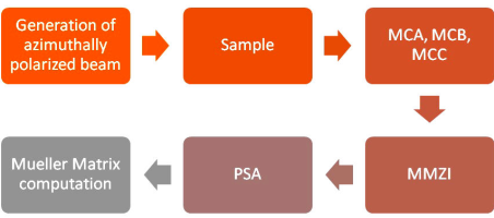
Figure (1) shows a flow diagram of the steps required to configure the experimental procedure. The idea is just to generate an azimuthally polarized beam that impinges on the sample under study, and then analyze the outgoing modified polarization state. The azimuthally polarized beam is generated with the aid of a S-wave plate converter (Altechna, model RCP-515-06), after an incident linearly polarized state is transmitted (@532 nm). In the usual procedure, using conventional or spatially homogeneous polarization, the analysis is realized in the polarization contribution, with the spatial distribution being implicit within the own intensity registration. However, analysis associated to classical entangled polarization states, as it is the case of azimuthal polarization, implies analyzing both degrees of freedom, one independent from the other: spatial distribution and polarization state ¹³. This is done by analyzing the spatial contribution first, using a mode converter (MCA, MCB, MCC) and a modified Mach-Zehnder interferometer (MMZI). The second degree of freedom is determined using a polarization state analyzer (PSA), and finally, the Mueller matrix (MM) can be computed using the relationships shown in Eqs. (4-6) ^13,14.

A mode converter (MC) is a device that affects the spatial degree of freedom of a given mode, without any effect on the other degree of freedom, the polarization state. For example, a half-wave or π-mode converter with the fast axis set at 22.5° will rotate an incident diagonal Hermite-Gauss mode ψ+e^x to a horizontal Hermite-Gauss mode ψ10e^x ¹³.

Figure 1 Schematic diagram of the experimental procedure. 

When the device is changed by a quarter-wave or π/2-mode converter with the fast axis at 45°, a conversion between Laguerre-Gauss fundamental modes and Hermite-Gauss fundamental modes is achieved ¹³. In any case, the polarization state is not affected. A mode converter can be obtained by using a couple of cylindrical lenses of the same focal distance ¹². MCA represents a π/2-mode converter, MCB represents a π-mode converter, and MMC represents an open space, with no mode-converter present ¹³. The modified Mach-Zehnder interferometer (MMZI) is a Mach-Zehnder interferometer with an additional mirror placed at one of the two arms [14]. The role of the MMZI is just to separate the orthogonal spatially distributed modes ^13,15. The polarization state analyzer, PSA, is applied to analyze the polarization contribution associated to each spatially distributed decomposed mode. The simplest PSA configuration is obtained by using a quarter-wave plate and a linear polarizer.

Figure 2 represents the 16 intensity measurements required by Eq. (4) in order to obtain the complete MM, once the incident classically entangled polarized state (azimuthal beam) has been modified by the transparent sample. The PSA is set to analyze the contribution to horizontal (X), diagonal at +45° (+45°), and vertical (Y) linear polarizations, and to circular right-hand polarized light (R). Intensity measurements are made using a CMOS camera.

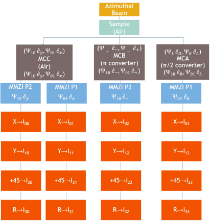
Figure 2 Schematic diagram of the required experimental intensity measurements to determine the Mueller matrix using a single azimuthally polarized beam of light @532 nm (following Ref. 13). 

The diagram in Fig. 2 explains the procedure to get the 16 experimental intensity measurements required for the determination of the Mueller matrix, according to Eqs. (4-6). Once the beam interacts with the sample, it passes through a mode converter A, B, or C. Each one of them will change the spatial distribution of the beam differently, but none of them will alter its polarization. For the case when the beam passes through MCC, which is air, its spatial distribution is conserved, and then it goes through the MMZI. The purpose of the MMZI is to decompose the beam into its orthogonal ψ10 and ψ01 modes (regardless of their polarization state) so, in this case, we will have mode ψ10 with its corresponding polarization e^y, at one port (say at port 1, P1), and mode ψ01, with polarization e^x, at port 2 (P2) (see Eq. (3.1)). At each output port, a PSA is placed, and we register the results from analyzing the horizontal (X→0), vertical (Y→1), +45° (+45°→ 2), and circular right-hand (R→3) polarizations with a camera. The intensities are taken from the images

which are labeled according to the polarization (first subscript) and the mode (ψ10→0, ψ01→1, ψ+→2 ψR→3, second subscript, as it is done in [13]).

The beam undergoes a similar procedure when it passes through MCB or MCA, with the difference that its spatial distribution will be affected differently, and that in such cases, we are interested in just one of the output ports of the MMZI (port 1), as their measurements correspond to the intensities required in Eq. (4).

Figure 3 is a detailed schematic representation of the experimental setup employed here, where the arrows show the modifications employed to get the three different mode converters (including the lenses required), in order to fulfill the analysis proposed in Fig. 2.

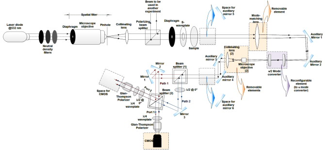
Figure 3 Schematic diagram of the proposed experimental setup for the determination of the Mueller matrix of a transparent sample using an azimuthally polarized beam of light. 

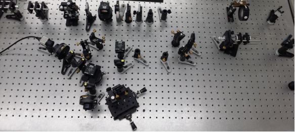
Figure 4 Experimental setup proposed here to determine the Mueller matrix using a single azimuthally polarized beam of light @532 nm (following Ref. 13). 

It is important to note that the original proposal ¹³ considers an optical arrangement such that the probe beam after the sample is split into three beams, which interact with the mode converters A, B and C at the same time, and then each beam goes through an independent MMZI. PSAs and photodetectors are placed at the output ports of each interferometer. It is implicitly considered that the cross-section of each beam is not affected.

In our arrangement, the beam interacts with each of these configurations in sequenced time, so we have space and mountings for removable elements, which allow us to adapt the experimental setup to each set of measurements.

The first step in our experiments is to generate the azimuthal beam. The illuminating source is a diode laser (@532 nm). We use neutral density filters, a spatial filter, a collimating lens, and a polarizing beam splitter (PBS) in order to obtain a homogeneous horizontally polarized collimated beam. The PBS is used as we employ the reflected beam into other independent setups. A diaphragm is used in order to experimentally control the diameter of the beam, as it is an important parameter for the mode-matching process required by MCA. The S-wave plate, adequately oriented, allows us to convert the horizontally polarized beam into the azimuthally polarized beam that is needed.

After the azimuthal beam has been generated, it interacts with the sample, and a lens with a focal length of 500 mm is placed to fulfill the mode-matching condition required by the π/2 converter ¹³. This element is called a mode-matching lens, as shown in Fig. 3. Auxiliary mirrors 1 and 2 send the beam to a pair of cylinder lenses that are adjusted to operate

in the MCA configuration, and then, a microscope objective and a lens are used to collimate the resulting beam. This beam is redirected with the help of auxiliary mirrors 3 and 4, in order to assure good alignment upon entering the MMZI. We place a camera after one PSA, make the measurement for one polarization state, and then change for the corresponding measurement at the other port. This allows us to be certain that we are registering both orthogonal modes (as they flip quickly between one port and the other with any minimal change in environment conditions). Once we have measured all the required polarization states for this mode converter, we proceed to implement MCB. For this purpose, we take out the mode-matching lens and the collimation system at the end of the cylinder lenses. We change the cylinder lenses for the π mode converter configuration (MCB), and follow the same steps as before to register the PSA results. For MCC, we place auxiliary mirror 5 right after the sample, and auxiliary mirror 6 in front of auxiliary mirror 4, in order to send the light directly to the MMZI (the beam does not change its cross-section size). The mode conversion operation is verified for each one of the mode converters. We register the PSA resulting images and proceed to their processing and analysis.

Figure 5 shows the best generated azimuthal polarization state through its image Stokes vector, where Figs. 5(a-d) represent s0, s1, s2, and s3, respectively (images taken after the S-wave converter, Fig. 3).

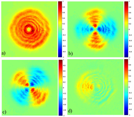
Figure 5 Imaging Stokes vector associated to the azimuthally polarized beam of light @532 nm, with spatial average symmetry hSi = [1 0.0455 0.0360 0.1187] ^T . 

A simple way to determine the quality of the beam generated can be provided by its spatial average symmetry (SAS) metric ¹⁶, which is the spatial average Stokes vector. For the case presented here, the spatial average Stokes vector is given by ⟨S⟩= [1 0.0455 0.0360 0.1187] T, which is interpreted as an unconventional polarization state with a slightly global tendency to a right-handed elliptical polarization state.

An ideal azimuthal polarization state has an associated spatial average Stokes vector equivalent to totally unpolarized light, ⟨S⟩= [1 0 0 0]T, ^13,16. Note there is a singularity at the center of each image; this is, in fact, a characteristic of any unconventional polarization with axial symmetry, as in the case of azimuthal polarization ^5,6,8,16.

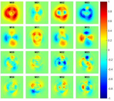
Figure 6 shows the normalized Mueller matrix obtained when the sample under study is the air.

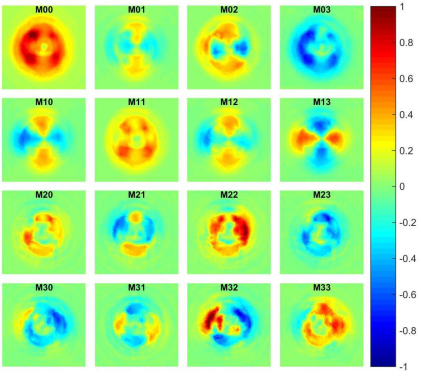
Figure 6 Imaging Mueller matrix associated to air, using a single incident azimuthally polarized beam of light (following Ref. 13). 

Ideally, Fig. 6 should be associated with a unitary imaging MM. Even when these images show this tendency, there are some deviations due to two main factors: the azimuthal polarization is not ideal, and the use of the mode converters implies the use of two cylinder lenses (for MCB) and, in addition, mode-matching lenses for MCA, which affect the intensity cross-section of the beams reaching the CMOS camera. These factors are present when Eqs. (4-6) are applied (following the intensity measurements according to Fig. 2) to obtain Fig. 6. Note that elements M00BW, M01BW, M10BW, M11BW, M20BW, M21BW, M30BW, M31BW (Eqs. 4-6) are determined by some of the intensity measurements (I00, I ₁₀ , I ₂₀ , I ₃₀ , I ₀₁ , I ₁₁ , I ₂₁ , I ₃₁ ) when there are no lenses present between the sample and the CMOS camera (MCC); intensities are added and subtracted for beams with the same cross-section size, and this is the reason why the results are close to the expected ones. Observe that the elements M02BW, M12BW, M22BW, M32BW are determined by the use of intensities where MCB (I ₀₂, I ₁₂, I ₂₂, I ₃₂) and MCC are present; the intensities are added according to Eq. (4), generating a mixture of slightly different cross-section sizes, which originates slight deviations from the expected results. Finally, note that elements M03BW, M13BW, M23BW, M33BW are associated with measurements where mode converters A and C are being present; this implies that these measurements are taken with the use of both, mode-matching and cylinder lenses for MCA (I ₀₃, I ₁₃, I ₂₃, I ₃₃) and no lenses for MCC, according to Eq. (4) and Figs. 2 and 3. These are the reasons for the deviations registered in relation to the expected results.

The results obtained for commercial thin film retarders of a half-wave and a quarter-wave retardance, with the fast axis set horizontally, are shown in Figs. 7 and 8, respectively. In addition to the goal of maintaining the same cross-section for all the beams measured, there are also some slight deviations associated to the true retardance shown by the wave plates at the incident wavelength (@532 nm). According to our measurements, the sample half-wave plate used causes a retardance of 161° (instead of the 180° expected), and the quarter-wave plate causes a retardance of 95.18° (instead of an ideal 90°) at this wavelength.

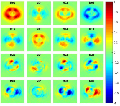
Figure 7 Imaging Mueller matrix associated to a half-wave plate with a horizontal fast axis, using a single incident azimuthally polarized beam of light (following Ref. 13). 

Figure 8 Imaging Mueller matrix of a quarter-wave plate with a horizontal fast axis, obtained using a single azimuthal incident polarization state (following Ref. 13). 

4. Conclusions

Inspired in a theoretical proposal ¹³, an experimental arrangement that uses a single classically entangled polarization state as incidence has been described for the determination of the imaging Mueller matrix. The open space and two wave-plate retarders have been used as the transparent samples under study. Results show that some experimental improvements are necessary in order to accurately implement the theoretical proposal on which this work is based. Three main factors have been identified as being inherently associated to experimental deviation from the ideal desired results: generation of a high quality azimuthal beam, control of the cross-section size for all the output beams coming from the different mode converters (which is to be the same), and control of the intensity of the beams entering the MMZI (which is also to be the same); that is, the main goal is just to get the same collimated beam after the sample and at the face of the CMOS camera. Also, since the MMZI is very sensitive, it is necessary to implement a real time stabilization system in order to get outputs that do not flip too quickly between ports. This, in addition to all the slight deviations in the delays caused by the non-ideal elements used in the experimental configuration, mainly the components of the MMZI which have important repercussions since, in order for the MMZI to exhibit a polarizing mode-splitter like behavior, elements with exact retardance of π are required ¹³, which are difficult to find in practice. Probably the use of plate beam splitters and a stabilized laser in both, intensity and frequency, could help to improve the final results.

We hope that the experiences derived from this work can contribute to accurately implement the theoretical proposal on which we have based this work ¹³.