Research
Research in Gravitation, Mathematical Physics and Field Theory
Wavelet characterization of hyper-chaotic time series
J.S. Murguíaa
H.C. Rosub
L.E. Reyes-Lópezc
M. Mejía-Carlosc
C. Vargas-Olmosc
a Facultad de Ciencias, Universidad Autónoma de San Luis Potosí (UASLP), Alvaro Obregón 64, 78000 San Luis Potosí, S.L.P., México.
b IPICyT, Instituto Potosino de Investigación Científica y Tecnológica, Camino a la presa San José 2055, Col. Lomas 4a Sección, 78216 San Luis Potosí, S.L.P., México.
c Instituto de Investigación en Comunicación óptica, UASLP, Alvaro Obregón 64, 78000 San Luis Potosí, S.L.P., México.
ABSTRACT
A wavelet scaling numerical characterization of time series based on the variance of the wavelet coefficients is used for three well-known four-dimensional and one five-dimensional hyper-chaotic systems. We report several scaling behaviors for the variables of these hyper-chaotic systems.
Keywords: Hyper-chaotic time series; discrete wavelet transform; wavelet variance; scaling analysis
RESUMEN
En este trabajo se realiza una caracterización de escala numérica de series de tiempo hiper-caóticas basada en la varianza de los coeficientes ondeleta de tres sistemas hiper-caóticos conocidos de cuatro-dimensiones y uno de cinco-dimensiones. Se reportan los diferentes comportamientos de escala de las variables de estos sistemas hiper-caóticos.
Descriptores: Series de tiempo hiper-caóticas; transformada ondeleta discreta; varianza ondeleta; análisis de escala
PACS: 05.45.-a; 05.45.Tp
1. Introduction
The wavelet transform (WT) is a mathematical tool for analyzing (decomposing) or synthesizing (reconstructing) a wide variety of generic signals at different frequencies and with different resolutions. In the wavelet analysis, a signal is decomposed into a type of functions called wavelets, which are translated and scaled versions of a finite-length and fast-decaying oscillating waveform. The latter is usually referred to as the analyzing wavelet basis function, or simply the mother wavelet. Similar to its preceding Fourier analysis, the wavelet analysis also contains various, closely-related forms of its transform, namely the continuous wavelet transform, the wavelet series, and the orthonormal discrete wavelet transform or, for short, the discrete wavelet transform (DWT). However, the most common choice to perform the analysis and synthesis of the original signal is the DWT because of the enormous versatility for computational calculations offered through its multiresolution filter bank structure1,2 . Just as in the other existent formats of the wavelet transform, the DWT is endowed with temporal resolution as a unique key advantage over its Fourier transform counterpart which allows to capture both the frequency and location information of the raw signal being processed in this way.
To the best of our knowledge, the class of hyper-chaotic systems, i.e., those dynamical systems having at least two positive Lyapunov exponents, have not been directly studied by means of wavelet transforms. This motivated us to provide here a wavelet scaling analysis of four hyper-chaotic systems, of which three are four-dimensional - Chen, Chua, and Rössler - and one is a recently introduced five-dimensional system. All these systems are reviewed in Sec. 2, where we briefly present their systems of equations and attractors for values of the parameters corresponding to the hyper-chaotic regime. Section 3 is devoted to a short description of the DWT. The main results are in Sec. 4, where we apply the wavelet analysis to the time series (TS) of the variables of these systems when they are in the hyper-chaotic regime. The paper ends up with a short conclusion section.
2. Hyper-chaotic systems
This section is devoted to a brief presentation of the four hyper-chaotic systems which we will consider in this work. These systems, despite their relative simplicity, exhibit a more complex dynamics than the chaotic systems, and they have received wide coverage in different areas of mathematics, physics, and engineering, among others3-9.
2.1. Hyper-chaotic Chen system
The hyperchaotic dynamics of Chen’s system is modeled by the set of differential equations4,6
x˙=a(y-x),y˙=x(d-z)+cy-w,z˙=xy-bz,w˙=x+k,
(1)
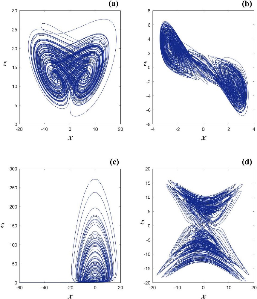
where a, b, c, d and k are parameters of the system. If a=36, b=3, c=28, d=-16 and -0.7≤k≤0.7, the system is in the hyper-chaotic regime. In fact, to check the existence of hyper-chaos, there must be at least two positiveLyapunov exponents. The numerically calculated exponents are λ1=1.627, λ2=0.060, λ3=0.000, and λ4=-12.684, which confirms such hyper-chaotic situation. In Fig. 1 (a), we display the hyper-chaotic attractor generated by the Chen system with k=0.5 projected onto the plane x-z.
2.2. Hyper-chaotic Chua system
We also consider the four-dimensional hyper-chaotic system based on Chua’s sytem as defined in Ref. 5
x˙=a(y-f(x)),y˙=x-y+z,z˙=-by-cz+w,w˙=-dx+yz,
(2)
with parameter values (a,b,c,d)=(30,50,0.32,0.1111), where the non-linear function f(x) is defined as the following cubic polynomial
f(x)=px+(1+q)x3,
(3)
with p=0.03 and q=-1.2. With the above-given value of d, we obtain the Lyapunov exponents λ1=0.529, λ2=0.017, λ3=0, and λ4=-12.221, which confirms the hyper-chaotic behavior. Figure 1 (b) shows one hyper-chaotic attractor projected on the plane x-z. It is worth to say that the spectrum of Lyapunov exponents depends on the parameter d, and we may obtain different attractors for other values of d5.
2.3. Hyper-chaotic Rössler system
This is the first system that has been shown to display hyper-chaotic behavior3. It is described by the equations
x˙=-(y+x),y˙=x+ay+w,z˙=b+xz,w˙=-cz+dw,
(4)
with parameter values (a,b,c,d)=(0.25,3,0.5,0.05), for which the corresponding four Lyapunov exponents are λ1=0.119, λ2=0.014, λ3=0, and λ4=-15.859. The x-z projection of the hyper-chaotic attractor for this system is shown in Fig. 1 (c).
2.4. A 5D hyper-chaotic system
The last case to be considered is a recent five-dimensional (5D) hyper-chaotic system defined in Ref. 7 and 8
x˙=a(y-x)+yzw,y˙=b(x+y)+v-xzw,z˙=-cy-dz-ew+xyw,w˙=-fw+xyz,v˙=-g(x+y),
(5)
with the values of the parameters (a,b,c,d,e,f,g)=(30,10,15.7,5,2.5,4.45,38.5). The corresponding five Lyapunov exponents are λ1=4.270, λ2=0.2501, λ3=0, λ4=-11.294, and λ5=-24.911. We can observe that its maximum Lyapunov exponent is larger than those of most hyper-chaotic systems, which implies more complex dynamic behaviors compared to other systems. Besides, there are cubic nonlinear product terms in four variables, while the order of other systems is usually not larger than two. Because of its significant complexity implying strong security, this 5D system has been considered in secure communication systems and cryptosystems7,8. Figure 1 (d) shows one projection of this 5D hyper-chaotic attractor.
3. The Discrete Wavelet Transform
In the DWT context, the representation of a generic function or process, x(t), is given in terms of the translated and dilated versions of the wavelet function, ψ(t), as well as its associated scaling function, φ(t)
1,2. Drawing on this principle and considering that the scaling and wavelet functions
φj,kt=2j/2φ2jt-k, ψj,kt=2j/2ψ(2jt-k), j,k=0,±1,±2,…
(6)
form an orthonormal basis, one can then write the expansion of x(t) as
x(t)=∑kakj0φj0,k(t)+∑j=j0J-1xkjψj,k(t),
(7)
where the scaling or approximation coefficients, akj, and the wavelet coefficients, xkj, are defined as
akj=∫x(t)φj,k(t)dt, xkj=∫x(t)ψj,k(t)dt,
(8)
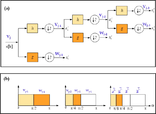
with j and k denoting the dilation and translation indices, respectively. To calculate akj and xkj in a practical numerical analysis, the DWT utilizes the so-called multiresolution analysis (MRA) approach. The key point of MRA is a multiscale, admissibility condition satisfying an approximation design originally developed by Mallat and Meyer2 whose theoretical foundation would ultimately develop into what is known as the fast wavelet transform (FWT). Consistent with this idea, the FWT algorithm connects, in an elegant way, wavelets and filter banks, where the multiresolution signal decomposition of a signal X, based on successive decompositions, is covered by a series of approximations and details which become increasingly coarser. As a result, a time-scale representation of a digital signal is obtained through the successive combinatorial coding of these digital filtering techniques. Briefly, the said procedure starts with the partitioning of the signal into an approximation and a detail part, which both together yield the original signal itself. This subdivision is such that the approximation signal contains the low frequencies, whereas the detail signal collects the remaining high frequencies. By repeatedly applying this subdivision rule to the approximation part, the details of increasingly coarse resolution are then progressively separated out while the approximation itself grows coarser and coarser. This procedure in effect offers a good time resolution at high frequencies and good frequency resolution at low frequencies, since it progressively halves the time resolution of the signal -signifying that only half the number of samples iteratively characterizes the entire signal- while gradually doubling the frequency resolution -since the frequency band of the signal spans only half the previous frequency band, effectively reducing thereby the uncertainty in the frequency by half as each decomposition level advances over. Figure 2 illustrates a typical three-level decomposition procedure of the FWT, panel (a), with the respective frequency decomposition bandwidth performed by the filters h[k] and g[k] in panel (b). Note that the bandwidth of the signal at every level is highlighted in a different color on each panel of the figure.
The FWT calculates the scaling and wavelet coefficients at scale j from the scaling coefficients at the next finer scale j + 1 by utilizing the following formulas
akj=∑lh[l-2k]alj+1,
(9)
xkj=∑lg[l-2k]alj+1.
(10)
In the above expressions, h[k] and g[k] are the low pass and high pass filters, respectively, in the associated analysis filter bank, whereas the signals akj and xkj are the convolutions of akj+1 with filters h[k] and g[k] followed by a down-sampling of factor 22, respectively. The wavelet transform, as many other available transforms, is reversible (i.e., it allows to go back and forth between the raw and processed signals), provided that the admissibility condition is satisfied; yet, it still exhibits high redundancy in the information it provides, significantly increasing the amount of computation time and resources for its processing. However, since the bandwidth filters utilized during the FWT process form orthonormal bases, the synthesis, or reconstruction, of the original signal can be conveniently performed by following in reverse order the above mentioned procedure, signifying a meaningful reduction in computation time. In short, the reconstruction of the original scaling coefficients akj+1 can be made from the following combination of the scaling and wavelet coefficients at a coarse scale
akj+1=∑lh[2l-k]alj+g[2l-k]xlj ,
(11)
which corresponds to the synthesis filter bank, and represents the inverse of the FWT for computing Eq. (7). This part can be viewed as the discrete convolutions between the up-sampled signal akj and the filters h[k] and g[k]. In other words, by following an up-sampling of factor 2, the convolutions between the up-sampled signal and the filters h[k] and g[k] are calculated, essentially signifying that the number of levels depends on the length of the signal, e.g., a signal with 2L values can be decomposed into (L+1) levels. Fig. 2 (a) illustrates a typical three-level decomposition process of the FWT. The corresponding frequency decomposition performed by the filters h[k] and g[k] is shown in Fig. 2 (b).
3.1. Wavelet Variance
In the wavelet approach the fractal character of a certain signal can be inferred from the behavior of its power spectrum P(ω), which is the Fourier transform of the autocorrelation function and in differential form P(ω)dω represents the contribution to the variance of the part of the signal contained between frequencies ω and ω+dω. Indeed, it is known that for self-similar random processes the spectral behavior of the power spectrum is given by
P(ω)∼∣ω∣-β,
(12)
where β is the spectral parameter of the signal. In addition, the variance of the wavelet coefficients var {xkj} is related to the level j through a power law of the type10
var {xkj}≈(2j)-β.
(13)
This wavelet variance has been used to find dominant levels associated with the signal, for example, in the study of numerical and experimental chaotic time series11-13. In order to estimate β we used a least squares fit of the linear model
log2(var{xkj})=-jβ+(K+vj),
(14)
where K and vj are constants related to the linear fitting procedure. Processes or signals corresponding to 1<β<3 are known as the fractional Brownian motions, where β=2 corresponds to the classical Brownian motion. On the other hand, processes within the interval -1<β<1, are termed fractional Gaussian noises; for example the classical stationary Gaussian white noise is a special case with β=0
10,12,14. Equation (13) is certainly suitable for studying discrete chaotic time series, because their log variance plot has a well-defined form as pointed out in12,13. If the log variance plot shows a maximum at a particular wavelet level, or a bump over a group of wavelet levels, which means a high energy concentration, it will often correspond to a coherent structure or a fundamental carrier frequency. In addition, if the log variance of the wavelet coefficients plotted against level j shows a slope -β, thus the signal presents a fractal behavior, which is consistent with the statistically self-similar structure of the signal12. In general, the slope of a noisy time series turns out to be zero in the variance plot, therefore it does not show any energy concentration at specific wavelet level. In certain cases the slope of some chaotic time series has a similar appearance to that of Gaussian noise at lower wavelet levels, which implies that these chaotic time series do not present a fundamental carrier frequency at any wavelet level.
4. Results
In this section, the scaling dynamics of the above-mentioned hyper-chaotic systems is evaluated with the wavelet variance scaling analysis. The hyper-chaotic systems are simulated numerically with the classical fourth-order Runge-Kutta algorithm. To carry out the wavelet analysis, we use the Daubechies wavelet function db2. This wavelet function possess several desirable properties such as orthogonality, approximation quality and numerical stability1,2. Also, the algorithm with the Daubechies family wavelet functions is memory efficient and is reversible, whereas other wavelet bases have a slightly higher computational overhead and are conceptually more complicated.
For our illustrative analysis, we first examine the hyper-chaotic Chen’s system (1). Figure 3 (a) shows a part of the TS of the z variable, whereas Fig. 3 (b) displays a semi-logarithmic plot of the wavelet coefficient variances as a function of level j, which is known as the variance plot of the wavelet coefficients. One can notice that the whole series is dominated by the 9th wavelet level, i.e., the major share of signal energy goes into this wavelet level. However, to catch almost the entire energy, we add together the six neighbor wavelet levels, j=6-11. The reconstruction of the signal at these wavelet levels is shown in Fig. 3 (c), where the structure of the original signal can be noticed. A similar behavior occurs in the TS of the x and y variables.
On the other hand, a different situation occurs for the TS of the w variable, which is shown in Fig. 4 (a). The logarithmic variance plot of its wavelet coefficients is displayed in Fig. 4 (b), where the line of negative slope indicates a fractal behavior. The fractal coefficient is given by the slope and its numerically calculated value is β≈2. This implies that this variable is statistically self-similar and corresponds to the classical Brownian motion. Such a situation does not occur in the case of chaotic time series of 3D chaotic systems12,13.
The second hyper-chaotic system that we study is Chua’s system . In this case, the first 17,000 TS samples of the z variable are shown in Fig. 5 (a), while the wavelet variance plot is given in Fig. 5 (b), where the behavior suggests a substantial energy concentration. We have found that by summing over the wavelet levels from j=5 to j=13 we are able to have a good reconstruction of the corresponding TS with the mentioned wavelet levels, see Fig. 5 (c). However, more than a half of the wavelet levels number is considered, which means that no significant energy concentration can be seen. Thus, this case does not have a fundamental carrier frequency and therefore this hyper-chaotic attractor has a Gaussian noisy behavior. A similar behavior is found for the TS of the x variable. The TS of the y variable required three wavelet levels less, which points to a fundamental carrierfrequency. As in the previous case, the TS of the w variable (Fig. 6 (a)) presents a similar fractal behavior in the majority of the high wavelet levels with a value of β≈2.3, as displayed in Fig. 6 (b).
Next, the hyper-chaotic Rössler system is analyzed. Figure 7 (a) displays a part of the TS of the z variable, and Fig. 7 (b) illustrates the wavelet variance plot. We notice a substantial energy concentration from the 9th to the 13th wavelet levels. Based on this range of levels, the reconstructed TS is shown in Fig. 7 (c). A similar situation occurs with the x and y variables. The latter results suggest again that a fundamental carrier frequency is present in these variables. On the other hand, the TS of the fourth variable, w, (Fig. 8 (a)), presents a fractal behavior in the high wavelet levels with a value of β≈1.6, as can be seen in Fig. 8 (b). The main result regarding this system is that it also presents two scaling behaviors as the previous hyper-chaotic systems do.
Finally, the scaling analysis of the 5D hyper-chaotic system shows that it presents also two different scaling behaviors in its TS, but the fractal behavior dominates in the majority of the TS of the variables. In the variance plot of the first two variables, x and y, the slope is close to zero, which means no significant concentration of energy. Thus, these variables do not present a fundamental carrier frequency, and therefore a Gaussian noisy behavior is present. But more interestingly, a fractal behavior is also observed in the rest of the variables, z, w and v, which is displayed in Fig. 9. The β values for the z and w variables are closer to the Brownian motion than the value obtained for the v variable.
As a summary, Table I shows the numerical results of
the wavelet variance analysis of the time series of all studied hyper-chaotic
systems. It is worth to say that the scaling parameter β is also related to other exponents, such as the scaling exponent α of the detrended fluctuation analysis (DFA) of the signal by α=(1+β)/2. With the β values obtained for the TS with fractal behavior, the corresponding
scaling exponents α are in agreement with those found in Ref. 15, which were calculated with a DFA method based on wavelets16. In addition, in Ref. 13 some chaotic systems were analyzed, but
the results showed that some variables present an energy concentration or Gaussian
noise behavior, whereas in this study we found that in the fourth variable a fractal
behavior can be present. Thus, with these new spectral properties may allow us to
have a better understanding of these kind of systems.
Table I Wavelet variance analysis of the TS of the hyper-chaotic systems. CF, GN, and F stand for carrier frequency, Gaussian noise, and fractal behaviors, respectively.
| Hyper-chaotic system |
Variables |
| x |
y |
z |
w |
v |
| Chen |
CF |
CF |
CF |
F |
- |
| Chua |
GN |
CF |
GN |
F |
- |
| Rossler¨ |
CF |
CF |
CF |
F |
- |
| 5D |
GN |
GN |
F |
F |
F |
5. Conclusions
In this work, the variance of the wavelet coefficients is used to analyze hyper-chaotic time series from different systems. It appears that the wavelet approach is a very illustrative means of revealing some dynamical properties of the hyper-chaotic systems. The results show a tendency of the majority of the time series of the variables of the 4D systems to present an enhanced energy concentration in a few wavelet levels, which we interpret as the carrier frequencies of the hyper-chaotic time series. On the other hand, for the fourth variable, a Brownian motion behavior is observed for the majority of the time series. For the time series of the 5D hyper-chaotic system, we have found a fractal behavior, closer to the Brownian motion behavior, in the time series of three variables (z, w, and v), with a nearly zero slope of the log variance of the wavelet coefficients at lower scales. This situation is different from the 4D hyper-chaotic systems. Finally, the information provided by this wavelet scaling analysis may be used to choose the appropriate hyper-chaotic dynamical system for whatever application.
Acknowledgements
LERL and CVO are CONACyT master and doctoral fellows, respectively, at FC-IICO-UASLP.
REFERENCES
1. I. Daubechies, Ten Lectures on Wavelets (Society for industrial and applied mathematics, 1992).
[ Links ]
2. S. Mallat, A Wavelet Tour of Signal Processing, 2nd. Edition (Academic Press, 1999).
[ Links ]
3. O. E. Rössler, Phys. Lett. A 71 (1979) 155.
[ Links ]
4. T. Gao, Z. Chen, Z. Yuan, G. Chen, Int. J. Mod. Phys. C 17 (2006) 471.
[ Links ]
5. P. C. Rech, H. A. Albuquerque, Int. J. Bif. and Chaos 19 (2009) 3823.
[ Links ]
6. T. Gao, Z. Chen, Phys. Lett. A 372 (2008) 394.
[ Links ]
7. B. Fan, L.R. Tang, 9th
International Conference on IEEE (2012) 2069.
[ Links ]
8. H.-M. Yuan, Y. Liu, T. Lin, T. Hu, L.-H. Gong, Signal Processing: Image Communication 52 (2017) 87.
[ Links ]
9. C. Li, J. C. Sprott, W. Thio, H. Zhu, IEEE Trans. on Circuits and Systems II: Express Briefs 61 (2014) 977.
[ Links ]
10. G.W. Wornell and A.V. Oppenheim, IEEE Trans. Inform. Theory 38 (1992)785.
[ Links ]
11. E. Campos-Cantón, J. S. Murguía, H. C. Rosu, Int. J. Bif. and Chaos 18 (2008) 2981.
[ Links ]
12. W. J. Staszewski, K. Worden, Int. J. Bif. and Chaos 3 (1999) 455.
[ Links ]
13. J.S. Murguía, E. Campos-Cantón, Rev. Mex. Fís. 52 (2006) 155.
[ Links ]
14. J. S. Murguía, H. C. Rosu, A. Jimenez, B. Gutiérrez-Medina, J. V. García-Meza, Physica A 417 (2015) 176.
[ Links ]
15. J. S. Murguía, Int. J. Mod. Phys. C. 28 (2017) Article 1750094.
[ Links ]
16. J. S. Murguía, J. E. Pérez-Terrazas, H. C. Rosu, Europhys. Lett. 87 (2009) 28003.
[ Links ]


 nueva página del texto (beta)
 Inglés (pdf)
 Artículo en XML
 Referencias del artículo
 Enviar artículo por email
 Citado por SciELO
  Similares en
SciELO
Similares en
SciELO 
 Permalink