SciELO - Scientific Electronic Library Online

 
vol.63 issue6Distribution of charge particles confined between three interfacial surfacesEntropía de discos rígidos auto-impulsados como parámetro de orden para peatones en contraflujo author indexsubject indexsearch form
Home Pagealphabetic serial listing  

Services on Demand

Journal

Article

Indicators

Related links

  • Have no similar articlesSimilars in SciELO

Share


Revista mexicana de física

Print version ISSN 0035-001X

Rev. mex. fis. vol.63 n.6 México Nov./Dec. 2017


Research

The 1-dimensional confined harmonic oscillator revisited

N. Aquino1 

E. Cruz1 

1Departamento de Física, Universidad Autónoma Metropolitana-Iztapalapa, Av. San Rafael Atlixco 186, Col. Vicentina, 09340, Ciudad de México, México. e-mail: naa@xanum.uam.mx


Abstract

We study the size effect on the energy levels of the 1-dimensional harmonic oscillator confined within a box of with impenetrable walls and large L. We use the particle in a box basis set to diagonalize the Hamiltonian of the confined harmonic oscillator. In this way we obtain the energy eigenvalues and eigenfunctions as a functions of L. We compare our numerical results with those reported in literature finding good agreement with the exact ones.

Keywords: Confined harmonic oscillator; energy eigenvalues; linear variational method

PACS: 03.65Ge; 02.60.-x

1. Introduction

The idea of the spatial confinement of quantum systems has gained growing interest in recent years due to its potential ability to model a great number of applications in different areas of Physics and Chemistry, as it is shown in several reviews and books1-8.

A spatially confined quantum system is defined as that in which its state functions satisfy certain boundary conditions for a finite value of the spatial coordinates1. The one-dimensional (1-D) harmonic oscillator limited by impenetrable walls is called 1-D confined harmonic oscillator (CHO).

The 1-D confined harmonic oscillator has been used as a model to study some more complicated systems, as for example: the proton-deuteron transformation to generate energy in dense stars9-10; in the theory of white dwarfs11, in the escape velocity of a star from a galaxy or a globular cumulus12; in the calculation of the specific heat of a crystal subjected to high external pressures14; in magnetic properties of metals15; in the study of color centers. More recently, the dynamics of a CHO subjected to a static electric field and a strong laser field has been studied39, it has called attention because it could be used to understand some aspects of the dynamics of ions caught in a Paul trap and in the study of the time of the revival of a particle in a CHO. Also few studies have been made on the transition probabilities and Einstein coefficients of the 1-D confined harmonic oscillator20,34,35 as a function of the box size, showing that new allowed transitions appear as a result of the confinement, this fact may be of technological interest.

Perhaps the first ones who studied the problem of the 1-D confined harmonic oscillator were Kothari andAuluck9-11. In the decade of the 40’s. They found that the eigen-functions of the system could be written in terms of Kummer’s functions. To obtain the values of the energy they needed to find the zeroes of the confluent hypergeometric function. They decided to carry out expansions and approaches to the hypergeometric function to obtain an analytical expression for the energy as a function of box size. They found the correct qualitative behavior; the energy of the levels of the CHO increases fast as the size of the box diminishes. Few years ago Baijal and Singh decided to get the zeroes of the hypergeometric function in a numerical way but their results were not accurate. Vawter improved the numerical results found by Baijal and Singh . At the beginning of 1980, Aguilera-Navarro et al. used the linear variational method to find, in a numerical way, the eigen-energies and eigen-functions of the CHO problem. They diagonalized the Hamiltonian matrix in the basis set of the free particle in a box of impenetrable walls. They obtained numerical values more accurate than those reported previously. However, the accuracy of their results is lower than the number of decimals that they reported.

The purpose of this work is to show the way in which the results of Aguilera-Navarro et al.30 can be improved.

The content of this work is as follows: In Sec. 2 we present the exact solution of the CHO problem. In Sec. 3 we use the linear variational method to obtain the energy eigenvalues. Finally, in section 4 we discuss our results and we give our conclusions.

2. The exact solution

The Schrödinger equation for the free 1-D harmonic oscillator (in natural units, m=ω==1) is given by

-12d2dx2+12x2ψ(x)=Eψ(x), (1)

where the unit of the distance is /mω and the energy is in units of ω.

In order to find the solutions of Eq. (1) we make the following substitution

ψ(x)=f(x)e-12x2, (2)

where f(x) satisfies the following equation

d2f(x)dx2-2xdf(x)dx+(μ-1)f(x)=0, (3)

where μ=2E.

Now we make a change of variable, by defining

ρ=x2, (4)

then the Eq. (1) is transformed to

ρd2f(ρ)dρ2+12-ρdf(ρ)dρ-14(1-μ)f(ρ)=0. (5)

This equation is identified as the Kummer differential equation. Its general solution, in terms of x, is given by:

f(x)=a1F114(1-2E);12;x2+bx1F114(3-2E);32;x2, (6)

where a and b are constants and 1F1 is the hypergeometric function37,38.

The potential energy of Eq. (1) is a symmetric function of x, therefore the eigenstates of the Schrödinger equation have definite parity; odd or even.

ψ+(x)=Ae-x2/21F114(1-2E);12;x2,ψ-(x)=Be-x2/2x1F114(3-2E);32;x2, (7)

In order that the wave functions do not diverge as x±, the hypergeometric function must terminate, this fact requires that there exist some non negative integer n such that

E=n+12,n=0,1,2,3,.... (8)

On the other hand, the exact solutions for the 1-D confined harmonic oscillator are well known 91020212530 they are obtained as follows. When the harmonic oscillator is symmetrically confined in a box, of length L=2a, of impenetrable walls, the energy quantization results from the boundary conditions on the wave functions

ψ±(x=-a)=ψ±(x=a)=0. (9)

The eigen-energies are found as the successive roots of the following equations:

1F114(1-2E);12;a2=0,forevenstates1F114(3-2E);32;a2=0,foroddstates (10)

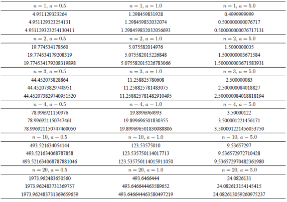
To determine the energy eigenvalues from these equations, it is necessary to solve numerically for one of the boundary conditions (4) according to the symmetry of the problem. The allowed energies can be determined with high accuracy by using some computer algebra system, Montgomery et al.16-17 used Maple but we can use Mathematica or a Fortran compiler with subroutines of extended precision. The numerical results obtained by solving the Eq. (5) with Mathematica 9 are reported in Table 1.

Table 1 Ground state energy for 1-D confined harmonic oscillator for few states n and different box sizes a. In the first row are the calculations of Aguilera-Navarro et al. 30. In the second row are the calculations of the present work, all calculations were carried out with N = 35 functions of the basis set. Finally, in the third row are the exact results obtained with the method described in the Sec. 2 and in the references16,17

3. Linear variational approach

The Schrödinger equation independent of time is given by

HΨ=EΨ. (11)

We use the linear variational method to solve the eigenvalue Schrödinger equation. The wavefunction Ψis expanded as

Ψ=i=1Nciϕi. (12)

where ci are constants to determine and ϕi is an orthonormal basis set.

The solution of eigen-value problem (Eq. 11) is equivalent to find the solutions of

(H-EI)c=0, (13)

where c=(c1,c2,c3,...,cN) is the vector of coefficients and I is the identity matrix, and

Hij=ϕi|H|ϕj, (14)

are the elements of the Hamiltonian matrix.

It is convenient to write the CHO Hamiltonian in the following way:

H=H0+H'. (15)

Where H'=(1/2)x2 and H0 is the Hamiltonian of a free particle in a box:

H0=p22+Vc, (16)

in which the potential is given by

Vc=0,x<a,x>a. (17)

The energy eigenvalues En0 and eigenfunctions ϕn of H0 are well known:

En0=n2π28a2, (16)

And

ϕn(x)=1/acos(nπx/2a),n=1,3,5,...1/asin(nπx/2a),n=2,4,6,.... (17)

The Hamiltonian matrix elements are:

Hij=Hij0+Hij', (18)

in which

Hij0=Ei0δij, (19)

where δij is the Kronecker delta.

The Hamiltonian H (Eq. 15) is symmetric, therefore its eigen-functions have definite parity, even or odd. For even (odd) states, the expansion in (Eq. 12) includes only even (odd) states as given by Eq. (19).

The matrix elements Hij' are analytical.

For even states they are:

Hij'={L2(-6+(1-2j)2π2)24(π-2jπ)2,ifi=j(-1)i+jL2(1(i-j)2-1(-1+i+j)2)4π2,ifij,i,j=1,2,3,. (20)

Whereas for odd states we have

Hij'={L248(2-3i2π2)ifi=j4ex(-1)i+jL2ij(i2-j2)2π2,ifij,i,j=1,2,3,. (21)

Where L=2a.

4. Results and discussion

The diagonalization of the CHO Hamiltonian was already employed by Aguilera-Navarro, Ley-Koo and Zimerman30 in 1980, and subsequently used again by Taseli and Safer36 at the end of the 90’s. In Table I we show the calculations obtained in the present work with those obtained by Aguilera-Navarro et al.30 and with the exact ones16. Our calculations were made by using Mathematica 9 with real variables with 25 decimal places. For comparison we used the same number of basis set, N=35, as Aguilera-Navarro et al.30.

We compare our results with the exact ones obtained by Montgomery et al.16,17, and we find that the present calculations have the precision shown in Table 1.

In Table I we can see that the accuracy in the calculations of reference30 is lower than the results of the present study. The reason for this difference is due to the fact that in the early 80’s the diagonalization subroutines were not as efficient and accurate as they are today, and it could also be due to the fact that the calculations with double precision real variables could only handle 16 decimal places.

As we can see there is an improvement in the accuracy of the energy eigenvalues for boxes with a<5. While for a=5 the accuracy of results of the present report and those of reference30 is the same. To improve the accuracy of the results of the present work it is necessary to increase the number of functions of the basis set to reach the exact results. In an Appendix we show the Mathematica procedure used to obtain the results presented in this work.

Acknowledgments

We thank S.A. Cruz, J. Garza and the two anonymous referees for their comments. E. Cruz thank CONACYT for the financial support through the scholarship 576678.

REFERENCES

1. F.M. Fernández and E.A. Castro, Kinam 4 (1982) 193. [ Links ]

2. P. O. Fröman, S. Yngve, N. J. Fröman, J. Math. Phys., 28 (1987) 1813. [ Links ]

3. S.J. Yngve, J. Math Phys. 29 (1988) 931. [ Links ]

4. W. Jaskólski, Phys. Rep., 271 (1996) 1. [ Links ]

5. A.L. Buchachenko, J. Phys. Chem. 105 (2001) 5839. [ Links ]

6. J.P. Connerade, V.H. Dolmatov and P.A. Lakshmi, J. Phys. B: At. Mol. Opt. Phys. 33 (2000) 251. [ Links ]

7. J.R. Sabin, E. Brändas and S.A. Cruz, Editors, Advances in Quantum Chemistry, vol. 57 and 58, (Academic Press, Amsterdam 2009). [ Links ]

8. K.D. Sen, Editor, Electronic Structure of Quantum Confined Atoms and Molecules, (Springer, New York 2014) [ Links ]

9. F.C. Auluck, Proc. Nat. Inst. Sci. India 7 (1941) 133. [ Links ]

10. D.S. Kothari and F.C. Auluck, Science and Culture 6 (1940) 370. [ Links ]

11. F.C. Auluck, Proc. Nat. Inst. Sci. India 8 (1942) 147. [ Links ]

12. S. Chandrasekhar, Astrophys. J. 97 (1943) 263. [ Links ]

13. E.M. Korson ad I. Kaplan, Phys. Rev. 71 (1947) 130. [ Links ]

14. N. Aquino, V. Granados and H. Yee-Madeira Rev. Mex. Fis. 55 (2009) 125. [ Links ]

15. R.B. Dingle, Proc. R. Soc. London A 212 (1952) 47. [ Links ]

16. H.E. Montgomery , N. Aquino and G. Campoy, Phys. Scr. 81 (2010) 045010. [ Links ]

17. H.E. Montgomery , G. Campoy and N. Aquino, Phys. arXiv:0803.4029V1[math-ph] 28 Mar 2008. [ Links ]

18. F.C. Auluck, Proc. Nat. Inst. Sci. India 7 (1941) 383. [ Links ]

19. F.C. Auluck and D.S. Kothari, Proc. Cambridge Philos. Soc. 41 (1945) 175. [ Links ]

20. J.S. Baijal and K.K. Singh, Progr. Theoret. Phys . (Kyoto) 14 (1955) 214. [ Links ]

21. T.E. Hull and R.S. Julius, Can. J. Phys. 34 (1956) 914. [ Links ]

22. S. Sengupta and S. Gjosh, Phys. Rev. 115 (1959) 1681. [ Links ]

23. K.K. Singh, Physica, 30, (1964) 211. [ Links ]

24. B. Suryan, Phys. Rev. 71, (1947) 741. [ Links ]

25. P. Dean, Proc. Cambridge Phil. Soc. 62 (1966) 277. [ Links ]

26. R. Vawter, Phys. Rev. 174 (1968) 749. [ Links ]

27. R. Vawter, J. Math. Phys. 14 (1973) 1864. [ Links ]

28. A. Consortini and B. R. Frieden, Nuovo Cimento 35B (1976) 153. [ Links ]

29. F.C. Rotbart, J. Phys. A: Math. Gen. 11 (1978) 2363. [ Links ]

30. V.C. Aguilera-Navarro, E. Ley-Koo and A.H. Zimerman, J. Phys. A: Math. Gen. 13 (1980) 3585. [ Links ]

31. F. M. Fernández and E. A. Castro, Phys. Rev. A 24 (1981) 2883;. [ Links ]

32. J. Garza, R. Vargas and A. Vela, Phys. Rev. E53 (1996) 1954. [ Links ]

33. J.L. Marín and S.A. Cruz, Am. J. Phys. 59 (1991) 931. [ Links ]

34. N. Aquino, E. Castaño, G. Campoy and V. Granados, Eur. J. Phys. 22 (2001) 645. [ Links ]

35. G. Campoy, N. Aquino and V.D. Granados, J. Phys. A 35 (2002) 4903. [ Links ]

36. H. Taseli and A. Zafer, Int. J. Quantum Chem. 61 (1997) 759. [ Links ]

37. NIST Digital library of Mathematical Functions, freely avalable at , Chapter 13;M. Abramowitz and I.A. Stegun, Handbook of Mathematical Functions, (Dover New York 1965) p.504. [ Links ]

38. J.B. Seaborn, Hypergeometric Functions and Their Applications, (Springer, New York, 1991) Chap. 3. [ Links ]

39. S. Lumb, S. Lumb and V. Prasad, J. Mod. Phys. 4 (2013) 1139. [ Links ]

appendix

(* Mathematica procedure to find the energy-eigenvalues *)

Clear ["Global*"]

delta[n_, m_] := KroneckerDelta[n, m](* Identity matrix*)

(* Even states *)

v[n_, m_] := 1/\[Pi]^2 (-1)^(m + n) a^2 (1/(m - n)^2 - 1/(-1 + m + n)^2) /; n != m ;(* non-diagonal elements of the harmonic oscillator potential (1/2)x^2 *) v[n_, m_] := (a^2 (-6 + (1 - 2 n)^2 \[Pi]^2))/(6 (\[Pi] - 2 n \[Pi])^2) /; n == m;(*Diagonal elements of the harmonic oscillator potential (1/2)x^2*)d[n_] := ((2 n - 1)^2 \[Pi]^2)/(8 a^2);(* Energy eigenvalues of a particle in a box*)

(* Odd states; replace the three functions defined before by the followin lines *)

v[n_, m_] := (4 (-1)^(m + n) a^2 m n)/((m - n)^2 (m + n)^2 \[Pi]^2) /; n != m ;

v[n_, m_] := 1/12 a^2 (2 - 3/(n^2 \[Pi]^2)) /; n == m;

d[n_] := ((2 n)^2 \[Pi]^2)/(8 a^2)*)

Hnm[n_, m_] := SetPrecision[N[ (d[n]) (delta[n, m]) + v[n, m], 25], 25];(* Hamiltonian matrix *)base = 35;(* Number of functions of the basis set *) matrizH = Table[Hnm[n, m], {n, 1, base}, {m, 1, base}]

Print[TimeUsed[]] a = 0.2;(* Box lenght*)

energias = SetPrecision[Eigenvalues[matrizH], 25];(* Energy eigenvalues*)

Sort[SetPrecision[energias, 25]]

Received: June 19, 2017; Accepted: August 11, 2017

Creative Commons License This is an open-access article distributed under the terms of the Creative Commons Attribution License