1. Introduction

Recently in¹, a methodology of optimization was applied to an irreversible Carnot-like power plant, where the characteristic parameters were: the allocation or effectiveness of the heat exchangers of this plant. Although this methodology is applicable to any Carnot-like power plant, a standard irreversible Carnot-like cycle was chosen because of its simplicity to account for the main irreversibilities that usually arise in real heat engines²: “finite rate heat transfer between the working fluid and the external heat sources, internal dissipation of the working fluid, and heat leak rate between reservoirs”. The above standard irreversible Carnot-like cycle has been studied at length for many objective functions, different transfer heat laws and several characteristic parameters (see^2-24 for more details).

The maximum power and efficiency have been obtained in^3-6. In general, these optimizations were performed with respect to only one characteristic parameter: internal isentropic temperature ratio (x) including the time too¹⁸. However, Bejan and Lewins^15,20 have considered the optimization with respect to other parameters (see also the reviews of^17-18 for more details): “the allocation, cost and effectiveness of the heat exchangers of the hot and cold sides”. On the other hand, effects of heat transfer laws or when a property is independent of the heat transfer law for this Carnot-like cyclic model, have been discussed in several works,^18-23, and so on.

On the other hand, n-stage combined Carnot cycle has been presented, by the law of heat conduction, in^24-26 optimizing the specific power and efficiency for the characteristic parameters: isentropic temperature ratios , and effectiveness (other combined cycles can be found in^27-36, coupled heat devices in^37-38; see also the references therein included).

In this paper we extend the results of allocation or effectiveness for one cycle to two or more combined cycles of the same irreversible Carnot-like power plant using iteratively the Bellman’ Principle³⁹ which has been successfully applied in Refs. ¹³ and ¹⁴. We found optimal recurrence relations remarkable for the irreversible power plant with n Carnot-like cycles for two constraints (design rules): constrained internal thermal conductance or fixed total area of the heat exchangers from hot and cold side.

This paper is organized as follows. In Sec. 2 we present the irreversible power plant model and the functional relation between power and efficiency which extends to the corollary presented in¹ to the irreversible power plant. Section 3 presents the optimization of the allocation and effectiveness, by two design rules, of heat exchangers for the Carnot-like 𝑛-cycles of the power plant. Section 4 is devoted Conclusions.

2. Power plant with n Carnot-like cycles

The power plant with n Carnot-like cycles is shown in Fig. 1. Each cycle satisfies the conditions expressed in^2,4: leak heat rate Q and finite heat transfer rates Q_i and internal dissipations of the working fluid expressed by constants Ii(i=1…n) such that Ii=(ΔSi+1/ΔSi)≥1;i=1…n ⁴ which make the Claussius inequality to become equality (for more details see^1,24). Each cycle of the power plant consists of two isothermal and two adiabatic processes. Denoting, for each cycle, the temperatures of the working fluid in the hot and cold isothermal processes as T2i-1 and T2i(i=1…n), respectively, and the end temperatures as T_H and T_L.

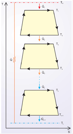
Figure 1 A power plant with n Carnot-like cycles, with heat leak rate, finite heat transfer rates, and internal dissipations of the working fluid in each cycle. 

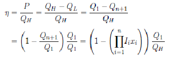
Following to^1,25, the thermal efficiency of the power plant is given by (this functional form for only a cycle has appeared in Refs. ¹, ², and ¹⁷):

where i=T2i/T2i-1 corresponds to the isentropic temperature ratio for each cycle i(i=1,....,n), P is the power of the plant, Q is the leak heat rate and the function

The Eq. (1) is obtained of the following way: according to the second Law of the Thermodynamics, for each i(=1,2,...,n), we have (cfr. With²⁵),

Thus,

Now, using the Eqs. (3) and (4), the efficiency is given by,

(5)

From the Eq. (5), Q1 is equal to:

And from the Eq. (6), (1) is obtained.

The Eq. (1) extends to the Eq. (6) of¹. Therefore, we can seek, as in¹, invariant optimal relations, by following the spirit of Carnot’s work, for other characteristic parameters, which can be independent from the heat transfer law, of the irreversible power plant.

Also, the Eq. (1) say us that it is enough analyzes only for power and efficiency (for other operation regimes, e.g. algebraic combination of power and/or efficiency that have thermodynamic meaning and satisfy imposed power conditions: see Eq. (7) below and for more details see¹). For instance, the functional expression of the efficiency, power and the heat transfer, without require of algebraic explicit expressions, have been used in², for two constraints (design rules): constrained internal thermal conductance or fixed total area of the heat exchangers from hot and cold side. The isentropic temperature ratio do not has this condition^{1,2,3,13,24-26}.

Now, if we take z≠xi(i=1,2....n) as other independent variable the Corollary given at¹ can be paraphrased as:

“The power 𝑃 achieves a maximum value in 𝑧 𝑚𝑝 if and only if the efficiency 𝜂 achieves a maximum value in the value: zmp=zme”

Thus, in the optimization of power plant, with respect to 𝑧 it is enough to find the maximum power by,

The optimization performed, with respect to will be: a property independent from the heat transfer law. This a remarkable conclusion of the Eq. (1) is that it can find the maximum for one and only one the power (see the criterion of²). For example the power, for power plant model, by

We show the above as follows: Let z≠xi(i=1,2....n) and the vector x=(x1,....,xn) and zmp the point in which the power achieves a maximum value, then,

The power and the efficiency satisfy the functional relationship given by the Eq. (1). Deriving (1) with respect to:

since, we can suppose that Q does not depend of the variable z.

Therefore,

where zme is the point in which the efficiency η achieves a maximum value which implies that their roots are the same zmp=zme. Also, it is easily seen that for zmp=zme, the efficiency reach a maximum since

In all the above calculations none transfer heat law has been used.

Therefore, it is enough to have one, and only one, algebraic expression of the power and any heat transfer law. We choose for our convenience the power and the conduction heat transfer Law since they are algebraically the simplest. In the optimization of the power of the plant for two constraints (design rules): constrained internal thermal conductance (z=ϕ) or fixed total area (z=ψ) of the heat exchangers from hot and cold side of the heat exchangers from hot and cold side.

3. Universal optimal relations for the allocation and effectiveness of the heat exchangers of the power plant

The optimization of power and efficiency with respect to is well known for combined cycles^13,24-26. Henceforth, x will be fixed and we will assume that the law of heat transfer rate can be any law, included also the heat leak rate. Essentially, we will treat the following two design rules: internal thermal conductance fixed; or areas fixed for heat exchangers; which will be applied alternatively.

The first design rule is that the internal conductance of the Carnot-like cycle is constrained to: ∑i=1nαi=Γ; where Γ is a constant, which is applied to the allocation of the heat exchangers from hot and cold side with the same overall heat transfer coefficient U by unit of area A in both ends of the cycle i and αi,αi+1(I=1,2....n-1) are the thermal conductance correspondent to the finite heat transfers of the hot/cold sides for this cycle. Thus,

where A_i,A_i+1 are heat transfer areas on hot/cold sides of the cycle i(i = 1,2…n - 1).

Alternatively, the second design rule is that the total area is constrained by: ∑i=1nAi=A; where Ai, Ai+1 are heat transfer areas on cold and hot side for the cycle i. Now, the total area (A) is fixed, but when distributed it has distinct overall heat transfer coefficients and hence different effectiveness on each one of the hot and cold sides. As αi=UiAi (see ¹ and ¹²), then,

where Ui, Ui+1 are the overall heat transfer coefficients on cold/hot sides of the cycle i(i=1,2.....n). From the result of the Sec. 2, it is enough to found “The maximum power of each Carnot-like cycle i(i=1,2.....n) for the two design rules (11) and (12)”

Indeed, the dimensionless power output (Eq. (2.5) for one cycle in³) for each cycle i is given by:

here h (x_i) is a function which depends on the heat transfer law since xi=T2i/T2i-1 is the isentropic temperature ratio of the cycle i ([^{1,2,3,13,24-26}]); and i, αi+1 i(i=1,2.....n-1) are the thermal conductance correspondent to the finite heat transfers of the cold/hot sides for this same cycle.

Next, applying the Bellman’ Principle³⁹, in form iterative, we can obtain the optimal relations for the allocation of the heat exchangers of the power plant (Fig. 1). This principle will be applied as it is indicated in²⁰: “to state that every part of an optimum path is optimal”.

REFERENCES

1. G. Aragón-González, A. Canales-Palma, A. Galicia-León, and J.M. Rivera-Camacho, J. Energy Inst. 85 (2012) 201-208. [ Links ]
2. G. Aragón-González, A. Canales-Palma, A. Galicia-León, and J.M. Rivera-Camacho, J. Phys. A: Math. Theor. 42 (2009) 425205. [ Links ]
3. G. Aragón-González, A. Canales-Palma, A. Galicia-León and I.R. Morales-Gómez, Braz. J. of Phys. 38 (2008) 543-550. [ Links ]
4. J. Chen, J. Phys. D: Appl. Phys. 27 (1994) 1144-1149. [ Links ]
5. Z. Yan and L. Chen, J. Phys. A: Math. Gen. 28 (1995) 6167-6175. [ Links ]
6. G. Aragón-González, A. Canales-Palma, A. Galicia-León and M. Musharrafie-Martínez. J. Phys. D: Appl. Phys. 36 (2003) 280-87. [ Links ]
7. N. Cegonho and T. Domingos, J. Non-Equilib. Thermodyn. 30 (2005) 113-127. [ Links ]
8. L.G. Chen, J. Zhu, F. Sun, C.A. Wu, Appl. Energ. (2004) 78 305-13. [ Links ]
9. L.G. Chen, J. Li, F.R. Sun, Appl. Energ. 85 (2008) 52-60. [ Links ]
10. J.M. Gordon, J. Appl. Phys. 69 (1991) 1-7. [ Links ]
11. A. Bejan, Entropy Generation through Heat and Fluid Flow (Wiley, New York 1982). [ Links ]
12. A. Bejan, Advanced Engineering Thermodynamic (Wiley, New York 1988). [ Links ]
13. A. Bejan, Int. J. Heat Mass Transfer. (1995) 38 433-44. [ Links ]
14. A. Bejan, Entropy Generation Minimization (CRC Press, Boca Raton, FL 1996). [ Links ]
15. F.L. Curzon and B. Ahlborn, Am. J. Phys. 43 (1975) 22-24. [ Links ]
16. M.H. Rubin, Phys. Rev. A 15 (1979) 2094-2102. [ Links ]
17. K.H. Hoffman, J.M. Burzler and S. Shuberth, J. Non-Equilib. Thermodyn. 22 (1997) 311-355. [ Links ]
18. A. Durmayaz, O.S. Sogut, B. Sahin and H. Yavuz, Progr. Energ. and Combus. Sci. (2004) 30 175-217. [ Links ]
19. G. Aragón-González, A. Canales-Palma, A. Galicia-León and J.R. Morales-Gómez. Rev. Mex. Fis. (2006) 52 309-314. [ Links ]
20. J.D. Lewins, Int. J. Mech. Eng. Edu. 28 (2000) 41-46. [ Links ]
21. A. De Vos A. Am. J. Phys. 53 (1985) 570-573. [ Links ]
22. A. Calvo, A. Medina, J.M. Roco, J.A. White and S. Velasco, Phys. Rev. E 63 (2001) 0371021-5. [ Links ]
23. G Aragón-González, A Canales-Palma and A Galicia-León. J. Phys. D: Appl. Phys. 33 (2000) 1403-10. [ Links ]
24. J.D. Lewins, Int. J. Mech. Eng. Edu. (1999) 27 91-101. [ Links ]
25. J. Chen, J. Phys. A: Math. Theor. 3 (1998) 3383-3394. [ Links ]
26. S. Bandyopadhyay, N.C. Bera and S. Bhattacharyya, Energ. Convers. Manag. 42 (2001) 359-371. [ Links ]
27. L.G. Chen, F.R. Sun and W.Z. Chen, Energy The International Journal 20 (1995) 1049-1053. [ Links ]
28. L.G. Chen, C. Wu and F.R. Sun, Applied Thermal Engineering 17 (1997) 639-645. [ Links ]
29. L.G. Chen, F.R. Sun, C. Wu and J.Z. Gong, Applied Thermal Engineering 17 (1997) 629-637. [ Links ]
30. L.G Chen, H. Duan, F.R. Sun and C. Wu, Journal of Non-Equilibrium Thermodynamics 24 (1999) 280-290. [ Links ]
31. L.G. Chen, Y.H. Bi, F.R. Sun and C. Wu, International Journal of Thermal Science 38 (1999) 712-718. [ Links ]
32. L.G. Chen, S. Cao, C. Wu and F.R. Sun, International Journal of Power and Energy Systems (1999) 19 103-106. [ Links ]
33. L.G. Chen, F.R. Sun, C. Wu, N. Ni, International Journal of Energy, Environment and Economics, 9 (1999) 35-49. [ Links ]
34. L.G. Chen, C. Wu and F.R. Sun, Energy Conversion and Management, 39 (1998) 113-116. [ Links ]
35. K. Ma, L.G. Chen, and F.R. Sun , Academy Proceedings in Engineering Science, 34 (2009) 851-864. [ Links ]
36. L.G. Chen, D.L. Ni, Z.L. Zhang and F.R. Sun, Applied Thermal Engineering, 102 (2016) 447-453. [ Links ]
37. B. Jiménez de Cisneros and A Calvo Hernández. Phys. Rev. E 77 (2007) 041127 [ Links ]
38. B. Jiménez de Cisneros and A. Calvo Hernández, Phys. Rev. Letters 98 (2008) 130602. [ Links ]
39. R. Bellman, Applied dynamic Programming (Princeton 1962). [ Links ]
40. D. Gunderson, Handbook of Mathematical Induction: Theory and Applications CRC Press series on discrete mathematics and its applications (2011). [ Links ]
Appendix
For the second optimization of the first design rule, the constraint is now:
a2α1+α3Γ2=1
with a2=1+I1; Γ2=Γ-i=4nαi a constant and fixing the temperature Tj(j=4....n+1) and applying only for the second cycle. In parameterizing,
ϕ=α1Γ2;1-a2ϕ=α3Γ2
Similarly, in optimizing
1a2ϕ+I21-a2ϕ
with respect to ϕ; we obtain:
ϕ2=1a2+I2
Solving
1-a2ϕ2ϕ2=I2=α3α1
so,
α3=I2α1
and a3=1+I1+I2. Continuing of this form arrive us to the Eq. (14). We can show the relation (14) by Mathematical Induction
38. Indeed for n=2 is true. We suppose that for n = k is true and we must show for n=k+1. From the hypothesis of induction the following is fulfilled. For the k-th optimization, the constraint is now,
akα1+αk+1Γk=1
where ak=j=0k-1Ij. In parameterizing
ϕ=α1Γk;1-akϕ=αk+1Γk
In optimizing
1akϕ+Ik1-akϕ,
we obtain:
ϕk=1ak+Ik.
Solving,
1-akϕkϕk=Ik=αk+1α1.
Therefore,
αk+1=Ikα1
And
ak+1=j=0kIj
And the proof is complete. For the second optimization of the second design rule, the constraint is now,
a2A1+A3u2=A2
Where
a2=1+a1u1a1u1;u2=U1U3;A2=A-i=4nAi
is a constant and fixing the temperature Tj(j=4....n+1). In parameterizing,
ψ=A1A;1-a2ψ=A3A
a2=1+1a1U1.
From (13)
1a2ψ+1(1-a2ψ)u2,
the optimization with respect to ψ, gives,
ψ2=u21+a2u2
1-a2ψ2ψ2=1+u2(a2-1)1+a2u2
Thus,
A3=1+u2(a2-1)u2A1
Continuing of this form arrive us to the Eq. (15). In analogous form, the proof of the relations (15) can be carry out by Mathematical Induction.
Received: April 05, 2017; Accepted: August 07, 2017
Creative Commons License This is an open-access article distributed under the terms of the Creative Commons Attribution License