Levitation forces between a finite rectangular superconductor and a spherical magnet

Sosa, V.; Sosa, V.

Services on Demand

Journal

Article

Indicators

Cited by SciELO
Access statistics

Revista mexicana de física

Print version ISSN 0035-001X

Rev. mex. fis. vol.63 n.6 México Nov./Dec. 2017

Research

Levitation forces between a finite rectangular superconductor and a spherical magnet

V. Sosa¹

¹Universidad Autónoma de Yucatán, Facultad de Ingeniería, Av. Industrias no Contaminantes por Periférico Norte S/N, Apartado Postal 150 Cordemex, Mérida, Yuc., México. Permanent address: Cinvestav-IPN Unidad Mérida, Departamento de Física Aplicada, Apartado Postal 73 Cordemex, 97310, Mérida, Yuc., México. e-mail: victor.sosa@cinvestav.mx

Abstract

A model to describe the interaction between a spherical permanent magnet and a square superconductor in the mixed state was elaborated. The proposal is based on image dipole ideas as is the case of the Frozen dipole model that has been used in the literature. More precisely, a frozen dipole was put in the center of the superconducting sample; this dipole “was born" when the first critical field was reached in that position. This led to the attractive force magnet-superconductor in the penetrated-field state. In the description of the Meissner state, the demagnetizing field was not included in the calculation. Both vertical and horizontal forces are discussed.

Keywords: Superconducting levitation; analytical; force calculation

PACS: 74.20-z; 74.25.Ha

1. Introduction

Superconducting levitation is a fascinating phenomenon that offers the potential development of fast, superconducting flywheels for energy storage applications¹. To make these devices possible, it is necessary to have a reliable description of the complex interactions of the superconductor with an external axisymmetric magnetic field. Relevant advances have been made since the early model of Hellman et al.² According to that model, a point dipole (the magnet) induces an image dipole inside the superconductor, which is considered to fill in the space below an infinite plane, i.e., the superconductor has an infinite thickness. This way, the magnetic field at the interface superconductor/vacuum remains parallel to the surface of the sample. This condition describes the Meissner effect in the superconductor, i.e., the field expulsion. To describe the interactions between the magnet and the superconductor in the mixed state represents a major task. Next, two common methods are briefly discussed: the frozen dipole model³ and the Bean model⁴. In the first model a second point dipole is induced inside the superconductor, oriented in such a way that it always attracts the magnet. As the magnet descends on the superconductor and approaches the surface, the dipole approaches also from the other side. Once the magnet gets at the closest point to the superconductor, the dipole gets “frozen" and remains in a fixed position despite future displacements of the magnet. It is necessary to add more frozen point dipoles in order to reproduce the hysteresis observed in the behavior of the vertical force⁵. In the Bean model the idea is to study the local distribution of both the current density -whether dependent or independent of the internal magnetic field- and the magnetic field inside the superconductor subjected to an external (usually uniform) magnetic field. The total forces are calculated by summing up the contributions from the whole sample.

Several reviews on the superconducting levitation forces have been published, see for example the article of Hull⁶ or more recently, the excellent work of Navau et al.⁷.

As mentioned before, in the image dipoles model the superconductor is assumed to be infinitely thick. Under this hypothesis, the images lie inside the superconductor no matter how far the magnet is. But, for a superconductor thinner than the height of the magnet, this idea is not feasible. A description based on the ideas of the frozen dipole model is proposed in this paper. In order to justify the proposal, we performed some measurements in a real system and compare them with the calculations. Next, the data used to feed the theoretical model are presented.

2. Experimental

We used a YBa₂ Cu₃ O₇ (YBCO) sample doped with CeO₂ (0.5 wt.%) This superconductor was prepared and characterized at the Laboratorie CRISMAT (France). The procedure of fabrication and texturing is described in detail in⁸. The superconductor was isostatically pressed before texturing in a 20 mm diameter disk. The sample was extracted from the pellet by polishing it to form a rectangular prism having width 2R = 10 mm, length 2S = 10 mm and thickness L = 3.5 mm. The melt-textured superconductor has a critical temperature of 88.4 K and a critical current density of 6.5 X 10⁴ A/cm² at 77 K and zero field.

The experimental setup is shown in Fig. 1. The superconducting sample was put into a liquid nitrogen bath (zero field cooling). Then, a spherical magnet with its magnetization directed vertically, having a mass of 0.712 g and a radius of 2mm, was lowered by hand towards the center of the superconductor following a vertical path. Because of the repulsive force exerted by the superconductor, it was necessary to push firmly the sphere. The magnet was released after achieving a stable levitation, once the magnetic lines were pinned to the superconductor. A height of a = 3.5mm was measured in that position.

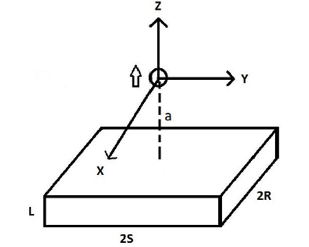
Figure 1 Experimental setup of the system. A spherical permanent magnet is placed above a rectangular superconductor, which was submerged into a liquid nitrogen bath (not shown). The centers of the sphere and the superconductor remain in the same vertical line. The center of the magnet is located a distance a above the upper surface of the rectangle. The empty arrow indicates the magnetic dipole moment μ of the sphere.

The magnet was previously characterized by measuring the magnetic field at different points along the symmetry axis, and it was concluded that it has a magnetic dipole moment μ=2.533×10-2 Am². The capability of the superconducting sample for trapping magnetic field was characterized in the following way. A permanent magnet was approached to the surface of the superconductor immersed in liquid nitrogen until their surfaces made contact; then, the magnet was retrieved. To estimate the trapped field in the superconductor, the field at the center of its upper surface (B _sc) was measured with a Hall probe. This was realized with different magnets wider than the YBCO sample. In every case, the field produced by the magnet (B _magnet) was measured at its surface and scanned over an area of 1x1 cm (the area of the superconductor). In order to have a representative field, the 30 measured values of B _magnet were averaged B _sc was measured in successive runs at least three times for every magnet and the values were averaged too. The results are shown in Table I.

Table 1 List of magnets used to magnetize the superconductor. Nd means a NdFeB magnet and Sm means a SmCo magnet. B _magnet is the average field applied to the superconductor in an area of 1 cm X 1 cm and B _sc is the magnetic field trapped in the sample.

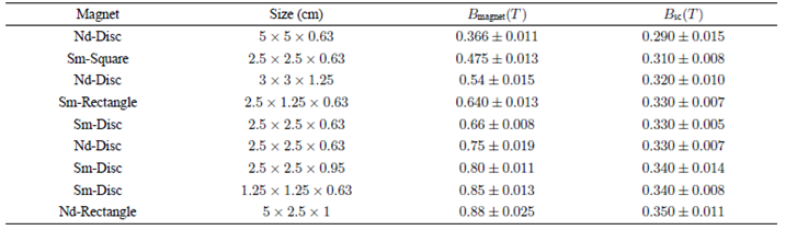
As B _magnet is increased, B _sc increases up to a value of 0.35 T. It is clear that the sample could trap higher fields if larger fields were applied. The capability of high-Tc superconductors for trapping magnetic fields has been studied extensively elsewhere⁹^,¹⁰. Now, the intention of including this characterization in this study was to compare the measured values of the trapped field with an estimation obtained with the model developed in the next section.

3. Theory

The force between a magnet and a superconductor in the mixed state will be described using two models: magnetic field full expulsion (Meissner state), Sec. 3.1, and penetration of the magnetic field, Sec. 3.2.

3.1 Field expulsion

First, the repulsive force between the magnet and a perfect diamagnet (i.e., a superconductor in the Meissner state) will be calculated. To perform this calculation it is necessary to know the magnetization of the superconducting sample, M(H _a), where H _a is the applied field. In the case of a complete field expulsion from the superconductor, we have B⃗=0, and therefore M⃗=-H⃗=-Ha⃗-HM⃗. Here, HM⃗ is the magnetic field produced by the superconductor with magnetization M⃗, i.e., the demagnetizing field. The following integral equation is obtained:

M⃗(r⃗)=-H⃗a(r⃗)-∫scdHM⃗. (1)

In principle, this equation might be solved by an iterative process. Usually, the magnetization of the superconductor is achieved by numerical calculations, mainly using the finite-element method¹¹^-¹³.

The intention of this work was to obtain full analytical expressions of the forces, but to calculate the demagnetizing field under a nonuniform external field H⃗a is a very complicated task. In a first approximation, the superconductor in Meissner state has a magnetization

M⃗(r⃗)=-H⃗a(r⃗). (2)

It will be shown that already, at this level, the model describes adequately the general characteristics of the system.

It is interesting to recall that according to the Bean model of the mixed state, the initial magnetization of an infinite superconducting slab of critical current density Jc and thickness L, when an external magnetic field is applied to it, can be written as M=-Ha+Ha2/Hp, where Hp=JcL is the so called penetration field. This expression is valid as long as Ha does not exceed Hp; Ha is assumed uniform and parallel to one of the sides of the superconductor. It can be seen that the assumption of neglecting HM⃗ in this work, leads to a similar conclusion when an infinite value of Jc is taken in the Bean model, in the sense that the same M⃗(Ha)⃗ is obtained in both cases.

The magnetization of a superconductor of orthorhombic shape in Meissner state has been previously studied theoretically and experimentally¹⁴. In that work, small samples of niobium (typically 1.5 mm X 1.5 mm X 1-to-6 mm) were subjected to a uniform external field H _a from 0 to 7×104 A/m. For low values of Ha, it was concluded that M=χHa χ is the initial susceptibility). For a superconductor with geometric proportions similar to the used in this work (width/length ≃ 0.35), their result is χ≃-2.5. As the ratio width/length of the superconductor growths, χ tends to -1, i.e., the demagnetizing field tends to disappear.

The force on the superconductor can be calculated by summing up all the infinitesimal interactions dF⃗ between each dipole dμ⃗=M⃗dV and the applied field B⃗a:

F⃗=∫sc∇(dμ⃗⋅Ba⃗)=μ0∫sc∇(dVM⃗⋅Ha)⃗=-μ0∫scdV∇(Ha)2 (3)

Here, the integration is taken over the whole volume of the superconductor. According to Eq. (3), it can be concluded that the force on the superconductor comes from a potential-energy density (dU/dV)=μ0Ha2.

This dipole-dipole model has been used previously to calculate levitation forces in different magnet-superconductor systems, e.g. dipole-cylinder¹⁵, bar-cylinder¹⁶, dipole-ring¹⁷, square-cylinder¹⁸, wire-sphere¹⁹, and ring-cylinder²⁰.

As shown in Fig. 1, the spherical magnet with dipole moment μ⃗ is located above a rectangular superconductor. The origin of the coordinate system is at the center of the magnet. The distance between this point and the upper surface of the slab is a. The center of the slab is located at (0,0,-(a+L/2)). The superconductor lies horizontal between the planes z=-a and z=-(a+L) with its sides parallel to the X and Y axes.

It is well known that the magnetic field due to a spherical magnet is the same as the one produced by a point dipole with the same magnetic moment located at the center of the sphere. This field is:

Ha⃗(r)=14π3r⃗(r⃗⋅μ⃗)r5-μ⃗r3 (4)

By substituting Eq. (4) in Eq. (3) and changing the sign, the repulsive force ejected on the magnet is obtained. Next, the vertical component of this force is calculated. Vertical μ⃗=μk^) and horizontal μ⃗=μi^ configurations were analyzed.

3.1.1 Vertical configuration

When μ⃗=μk^, the vertical force on the magnet is given by

Fz=μ04πμ216πg(a)-g(a+L) (5)

where g as a function of the independent variable ξ is defined as

g(ξ)=RSξ2(ξ2+R2)2(ξ2+S2)2(ξ2+R2+S2)2×[R6(9ξ2+6S2)+R4(35ξ4+41ξ2S2+12S4)+R2(48ξ6+80ξ4S2+41ξ2S4+6S6)+22ξ8+48ξ6S2+35ξ4S4+9ξ2S6+3R(7ξ4+10ξ2R2+4R4)ξ4(ξ2+R2)5/2arctanSξ2+R2+3S(7ξ4+10ξ2S2+4S4)ξ4(ξ2+S2)5/2arctanRξ2+S2 (6)

By taking S→∞, the expression for an infinitely long slab is obtained:

g(ξ)=3πR27ξ4+10ξ2R2+4R4ξ4(ξ2+R2)5/2 (7)

Furthermore, when R→∞, the result for an infinite sheet is obtained:

g(ξ)=6πξ4 (8)

Finally, if L→∞, the vertical force between the magnet and an semi-infinite superconducting plane results to be

Fz=μ04π3μ28a4 (9)

which is the early expression obtained by Hellman et al.² with the images method.

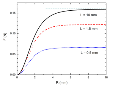
The variation of Fz with the dimensions of the superconductor is shown in Figs. 2 and 3. It can be seen that this force grows monotonically and reaches a saturation value. It is interesting to note that for a sample with 2R=2S=2 cm (about six times the distance to the magnet) and L=1 cm, the vertical force is practically the same as the one obtained for an infinite sample. This explains the success of Hellman’s model even for these small samples.

Figure 2 Vertical force (Eqs. (5) and (6)) on a spherical magnet with μ = 2:533 X 10^-2 Am ² as a function of the width of the rectangular superconductor in Meissner state. We took R=S for simplicity. The sphere is placed at a = 3:5 mm above the superconductor, with its magnetization along the z direction. The force grows monotonically and saturates at different levels, depending on the value of L. For a thickness of 10 mm and higher, the saturation force practically coincides with the result given by Eq.(9) for an semi-infinite sample (horizontal discontinuous line).

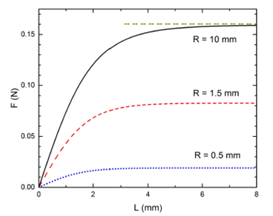
Figure 3 Vertical force (eqs. (5) and (10)) on a spherical magnet with μ = 2:533 X 10^-2 Am ² as a function of the thickness of the superconductor in Meissner state. Again, R = S, a = 3:5 mm and ¹ in the vertical direction. The force grows monotonically with L and reaches a saturation value which depends on R. The horizontal discontinuous line represents the value given by Hellman’s model for a semi-infinite superconductor.

3.1.2 Horizontal configuration

The result of Fz for μ⃗ oriented along the x direction in the same expression than Eq. (5), but in this configuration the function g(ξ) is given by

g(ξ)=RSξ2(ξ2+R2)2(ξ2+S2)(ξ2+R2+S2)2×3R6+6R4(2ξ2+S2)+ξ4(ξ2+S2)+R2(10ξ4+10ξ2S2+3S4)+3R(2ξ4+5ξ2R2+2R4)ξ4(ξ2+R2)5/2arctanSξ2+R2+3S(3ξ2+2S2)ξ4(ξ2+S2)3/2arctanRξ2+S2 (10)

For S→∞, i.e., an infinitely long slab:

g(ξ)=3πR(2ξ4+5ξ2R2+2R4)2ξ4(ξ2+R2)5/2 (11)

Now, by taking R→∞, the expression for an infinite sheet follows:

g(ξ)=3πξ4 (12)

Again, in the limit of a semi-infinite plane (L→∞) the vertical force tends to the value (μ0/4π)(3μ2/16a4), which coincides with the value obtained with the images method².

3.2 Field penetration

To describe the penetration of the magnetic field in the superconductor, an assumption is made based on the frozen dipole model. A magnetic point dipole represents the behavior of the penetrated region of the sample. This is equivalent to making a multipole expansion of the magnetic field and retaining only the dipole term. In the present model it will be assumed that the dipole appears and stays at the center of the sample. More precisely, the dipole appears in this point when the first critical field Hc is reached. After that, as the magnet keeps getting closer to the superconductor, the magnitude of the induced dipole moment μs increases until the magnet reaches the position where the mechanical equilibrium is reached. It is assumed that the magnetization of the magnet remains oriented vertically all its way. Therefore, the induced magnetic point dipole will be oriented always in the same direction.

The first critical magnetic field can be obtained from Hc(T)=H0[1-(T/Tc)2]. For an YBCO sample submerged in liquid nitrogen it will be taken H0=100 Oe, Tc=90 K and H=77 K, and obtain Hc(77k)=27 Oe. This value is reached at the center of the superconductor when the center of the magnet is located at a distance of 12.3 mm, i.e., when a=10.6 mm.

When the stable levitation of the sphere is reached at a=3.5 mm, the repulsive force given by Eqs. (5) and (6) must be equal to the weight of the magnet plus the force between the magnet and μs. This way the value μs=6.95×10-3 A m2 is obtained.

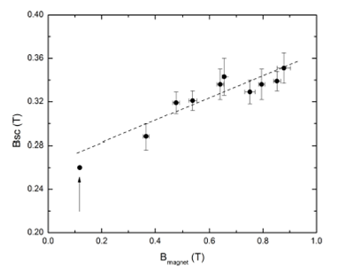
In order to evaluate how reasonable this value is, two fields at the center of the upper surface of the superconductor were calculated: the one due to the spherical magnet levitating at its equilibrium position, and the one produced by the induced dipole μs. These fields are 0.12 T and 0.26 T respectively. These two numbers were compared with the measured values of trapped field in the superconductor (Table I), as shown in Fig. 4. It is easy to see that the theoretical estimation fits nicely with the experimental trend.

Figure 4 Trapped magnetic field in the rectangular superconductor as a function of the magnetic field of the permanent magnets described in Table I. The data with error bars correspond to the experimental values reported there. The point signaled with an arrow corresponds to the calculated fields produced by the spherical magnet and the induced dipole μ_s at the upper surface of the superconductor. This theoretical point is in good agreement with the observed experimental behavior. The dotted line is a guide for the eye.

Based on the experimental observations, it is assumed that the magnitude μs varies from 0 to 6.95×10-3 A m² as the magnet descends to the superconductor. The precise dependence of μs with the height a given in mm (3.5<a<10.6), is assumed to have an exponential behavior:

μs(a)=6.95×10-3Am2(10.6-a7.1)n (13)

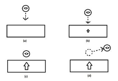
where n is an adjusting parameter. Following the idea of the frozen dipole model, it is assumed that when the magnet is moved apart from its equilibrium position, μs remains frozen at the center of the superconductor. This behavior is sketched in Fig. 5.

Figure 5 Diagram that illustrates the proposed mechanism of how the superconductor sample is penetrated by the magnetic field of the magnet. (a) No penetration occurs while a>10.6 mm (H_a < H_c ). (b) Once the critical magnetic field is reached, a magnetic dipole μ_s appears and stays at the center of the superconductor; μ_s increases when a diminishes, following Eq. (13); 3.5 mm < a < 0.6 mm. (c) μ_s reaches its maximum value when the magnet gets the position where the mechanical equilibrium is reached. (d) The induced dipole remains frozen (same value and same position) when the magnet is retrieved.

4. Total force

In this section the combined contributions of the repulsive and attractive forces on the magnet are analyzed. The force ejected by a magnetic dipole μ⃗ located at the origin on a second dipole μs⃗ located at point r⃗ is given in general by¹²:

Fs⃗=3μ04πr5(μ⃗⋅r⃗)μs⃗+(μs⃗⋅r⃗)μ⃗++(μ⃗⋅μs⃗)r⃗-5(μ⃗⋅r⃗)(μs⃗⋅r⃗)r2r⃗ (14)

In the vertical configuration of our geometry, μ⃗=μk^, μs⃗=μsk^, and r⃗=(x,0,z). Substituting in Eq. (14) and changing the sign, the attractive force ejected on the magnet is:

Fm⃗=3μ0μμs4π(x2+z2)5/25z2x2+z2-1xi^+5z2x2+z2-3zk^ (15)

4.1 Vertical

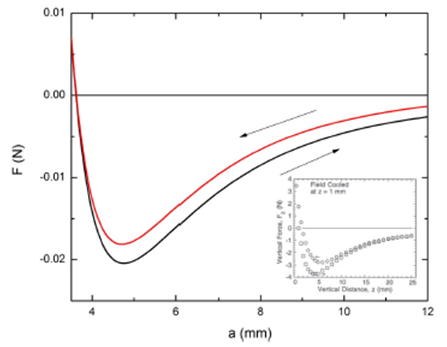
The total vertical force ejected by the superconductor on the magnet is the sum of the calculated from Eqs. (5)-(6) and the 𝑧 component of Eq. (15). In particular, the analysis will be restricted to the case x=0. As mentioned before, μs increases from 0 to its maximum value according to Eq. (13) during the descent of the magnet, and stays with the same value during the ascent. As Wu et al.⁵, we use the value n=0.8. As shown in Fig. 6, a typical hysteretic curve for a field cooling (FC) process is observed. The minor loops at intermediate points of the path were not considered in the model. It has been shown that these loops can be explained by adding more frozen dipoles in the superconductor⁵.

Figure 6 Total vertical force on the magnet as a function of the distance a, calculated with μ = 2:533 X 10^-2 A m², R = S = 5 mm, L = 3.5 mm, and n = 0:8. The weight of the magnet (= 7 X 10^-3 N) was not included. The arrows indicate whether the magnet approaches to (upper branch) or moves away from (lower branch) the superconductor. A typical hysteretic FC curve from Ref. ⁶ is shown in the inset, and a good qualitative agreement with the model is observed.

By the other hand, if n=5, we obtain a typical behavior for a zero field cooling (ZFC) process, as shown in Fig. 7.

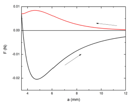
Figure 7 Total vertical force on the magnet as a function of the distance a, calculated with μ= 2:533 X 10^-2 A m², R = S = 5 mm, L = 3.5 mm, and n = 5. Again, the weight of the magnet was not considered here. The arrows indicate that the magnet approaches to and moves away from the superconductor (upper and lower branch, respectively). A typical hysteretic ZFC curve is observed.

4.2 Horizontal

When x=0, there is no horizontal force acting on the magnet. However, when it is displaced laterally along the X axis, the resulting horizontal force is the combination of the x-component in Eq. (15) and the repulsive force FP due to the Meissner state of the superconductor. The later was calculated starting from Eq. (3) using Mathematica, and the result is

FP=μ0μ2128π2P(R,S,-a,x)-P(R,S,-(a+L),x)+P(-R,S,-a,x)-P(-R,S,-(a+L),x) (16)

Where

P(α,S,z,η)=(zS3)3S2z2+[z2+(α-η)2](α-η)2[z2+(α-η)2]2(α-η)2-z2+S2[2+3z2S2+(α-η)2]+(α-η)2[S2+z2+(α-η)2]2+3S[2S2+3(α-η)2][S2+(α-η)2]3/2(α-η)4×arctan⁡zS2+(α-η)2+2α4+2z2-8α3η+5z2η2+2η4(α-η)4[z2+(α-η)2]5/2+α2(5z2+12η2)-2αη(5z2+4η2)(α-η)4[z2+(α-η)2]5/2×3zarctan⁡Sz2+(α-η)2 (17)

For an infinite sample (R,S,L→∞), the repulsive force tends to zero for any finite value of x, as it should be.

The total horizontal force Fx is shown in Fig. 8. It can be seen that for lateral displacements below 4.4 mm, the attractive force dominates over the repulsive one and the magnet is pulled to return to its equilibrium position. Above 4.4 mm, the repulsive force is higher than the attractive force and the magnet is pushed off. This result is particularly important to describe the stability of the magnet around its levitation position. The calculation is qualitatively in agreement with the experimental results²³^,²⁴. For x≪z ∣x∣≤ 1 mm), the force approaches the straight dashed line shown in Fig. 8. The slope of this line is k=50 N/m. This value is remarkably similar to the obtained by Johansen et al²² in their theoretical study of the lateral oscillations of a rectangular superconductor in the mixed state levitating on a rectangular magnet (k=56 N/m for a 3.5 mm separation). Neglecting the damping caused by friction, the magnet of mass 0.712g is expected to oscillate harmonically in this region with a frequency of 42 Hz. To verify this, the magnet was given a slight push and its further motion was monitored by measuring the magnetic field in a fixed point above the magnet, close to its equilibrium position. The variation of the field with time is shown in the lower inset of Fig. 8. It was observed that the magnet oscillated with a frequency of only 7 Hz, i.e., one sixth of the calculated value. This measurement was confirmed with a stroboscope. In order to consider the effect of the demagnetizing field on the magnetization in the Meissner state, the result for a superconducting rectangular prism under a uniform external field: M=-2.5Ha ¹⁴, was used instead of M=-Ha, Eq. (2). As a result, the theoretical frequency shifted to 39 Hz, still far from the measured value. Clearly, to improve the agreement it is necessary to take into account the damping of the motion and calculate the demagnetizing field of the superconductor under the specific nonuniform magnetic field of the magnet used in this study.

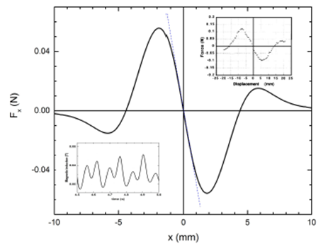
Figure 8 Total horizontal force (continuous line) on the magnet as a function of its position along the X axis. The data used in the calculation are: μ = 2:533 X 10^-2 A m², μ_s = 6:95 X 10^-3 A m², R = S = 5 mm, L = 3.5 mm, and a = 3.5 mm. The full curve is antisymmetric in x. The dashed straight line corresponds to a harmonic oscillator behavior. The upper inset shows experimental data taken from Ref. 23, which are in good agreement with the model. The lower inset shows the variation of the magnetic field measured at a fixed point, when the magnet oscillates horizontally around its equilibrium position.

5. Conclusions

The model proposed in the present work neglects the demagnetizing field but provides analytical expressions that describe several aspects of the force between a permanent magnet and a finite superconductor in the mixed state. More precisely, these issues are: i) The dimensions of the superconductor are incorporated in the calculation. In the limit of an infinite superconductor, the repulsive force tends to the proper value. This way, the model allows us to quantify how good/bad is the approximation of taking the sample as infinite. ii) The frozen dipole model was adapted to be applicable to a superconductor with finite thickness. The magnetic moment of this dipole was obtained from the condition of mechanical equilibrium observed experimentally. This value was consistent with our measurements of the magnetic field trapped in the superconductor. iii) The different ways in which the sample can be magnetized were parameterized by an exponent 𝑛. By varying this parameter it was possible to reproduce the typical hysteretic approach/draw-away curves of the total vertical force in FC and ZFC processes. iv) The total horizontal force was calculated as well, and a good agreement with previous experimental results was observed.

Acknowledgements

I want to acknowledge the financial support given by Conacyt (grant No. 245453) and the technical help of Dr. Fidel Gamboa and Osvaldo Gomez.

REFERENCES

1. F.N. Werfel et al., Supercond. Sci. Technol. 25 (2012) 014007. [ Links ]

2. F. Hellman, E.M. Gyorgy, D.W. Johnson Jr, H.M. O’Bryan, and R.C. Sherwood, J. Appl. Phys. 63 (1988) 447. [ Links ]

3. A.A. Kordyuk, J. Appl. Phys. 83 (1998) 610. [ Links ]

4. C.P. Bean, Phys. Rev. Lett. 8 (1962) 250. [ Links ]

5. Xing-da Wu, Ke-Xi Xu, Yue Cao, Shun-bo Hu, Peng-xiang Zuo, and Guan-dong Li, Physica C 486 (2013) 17. [ Links ]

6. J.R. Hull, Levitation Applications of High-Temperature Superconductors. In: A. V. Narlikar (ed.), High Temperature Superconductivity 2 - Engineering Applications (Springer Verlag, Berlin-Heidelberg 2004), pp. 91-142. [ Links ]

7. C. Navau, N. Del Valle, and A. Sanchez, IEEE Trans. Appl. Supercond. 23 (2013) 8201023. [ Links ]

8. C. Leblond, I. Monot, J. Provost, and G. Desgardin, Physica C 311 (1999) 211. [ Links ]

9. Z. Deng, K. Tsuzuki, M. Miki, B. Felder, S. Hara, and M. Izumi, Physica C 471 (2011) 1459. [ Links ]

10. M. Tomita and M. Murakami, Nature 421 (2003) 334. [ Links ]

11. E. Diez-Jimenez, I. Valiente-Blanco, and J.-L. Perez-Diaz, J. Supercond. Nov. Magn. 26 (2013) 71. [ Links ]

12. G. Iannone, S. Farinon, G. De Marzi, P. Fabbricatore, and U. Gambardella, IEEE Trans. Appl. Supercond. 25 (2015) 8200107. [ Links ]

13. I.A. Rudnev, A.I. Podlivaev, IEEE Trans. Appl. Supercond. 26 (2016) 8200104. [ Links ]

14. C. Navau, C.A. Cardoso, O.F. de Lima, and F.M. Araujo-Moreira, J. Appl. Phys. 96 (2004) 486. [ Links ]

15. J. Lugo and V. Sosa, Physica C 324 (1999) 9. [ Links ]

16. M.K. Alqadi, F.Y. Alzoubi, H.M. Al-Khateeb, and N.Y. Ayoub, Mod. Phys. Lett. B 20 (2006) 1549. [ Links ]

17. F.Y. Alzoubi, M.K. Alqadi, H.M. Al-Khateeb, and N.Y. Ayoub, IEEE Trans. Appl. Supercond. 17 (2007) 3814. [ Links ]

18. H.M. Al-Khateeb, M.K. Alqadi, F.Y. Alzoubi, and N.Y. Ayoub, Chinese Phys. Lett. 24 (2007) 2700. [ Links ]

19. H.M. Al-Khateeb, M.K. Alqadi, F.Y. Alzoubi, and N.Y. Ayoub, J. Supercond. Nov. Magn. 21 (2008) 93. [ Links ]

20. H.M. Al-Khateeb, F.Y. Alzoubi, M.K. Alqadi, and N.Y. Ayoub, Turk. J. Phys. 31 (2007) 271. [ Links ]

21. K.W. Yung, P.B. Landecker, and D.D. Villani, Magn. Electr. Separ. 9 (1998) 39. [ Links ]

22. T.H. Johansen and H. Bratsberg, J. Appl. Phys. 74 (1993) 4060. [ Links ]

23. T. Hikihara and G. Isozumi, Physica C 270 (1996) 68. [ Links ]

24. Yong Yang and Xiaojing Zheng, Supercond. Sci. Technol. 21 (2008) 015021. [ Links ]

Received: October 17, 2016; Accepted: July 25, 2017

This is an open-access article distributed under the terms of the Creative Commons Attribution License