PACS: 03.65.Fd; 11.80.Cr
1. Introduction
The use of the helicity, i.e. the projection of the spin along the direction of the momentum, to describe the polarization of Dirac particles in collision problems became common as a result of the pioneering work by Jacob and Wick 1. Obviously, the reason is that the energy eigenstates of the Hamiltonian are also helicity eigenstates. In particular the plane wave solutions of the free Dirac equation which are used to represent the incident and outgoing particles in the first order S-matrix are simultaneous eigenstates of the helicity operator Σ.P of the particle. The analysis of collisions with the use of these basis is greatly simplified.
Among the interactions that conserve helicity, probably, the interaction with a static magnetic field is the most popular. As is well-known, the helicity of a Dirac particle in an electromagnetic potential is conserved given that there is no electric field acting on the particle 2. Indeed, the Heisenberg equation of motion for the helicity operator Σ.Π where Π=(p-eA) is the mechanical momentum of the particle reads (ℏ=c=1):
Σ.Π,H=eΣ⋅E
(1)
Here, H is the Hamiltonian of a Dirac particle in an electromagnetic field. Thus, the helicity of a particle in a static magnetic field is conserved. In physical terms, conservation of helicity is described as the invariance of the component of the spin of the particle along its momentum. In the perturbative expansion of a helicity-conserving theory, helicity is conserved at each order of the perturbation series. For example, in the first order S-matrix element of the elastic scattering of a particle in some helicity-conserving vector potential, the conservation of helicity manifests itself through the fact that if the incident state is in an eigen state of the helicity operator Σ.p^i (p^i≡(pi/|pi|)), then the matrix element for the transition to a final state with the opposite helicity is zero 2 (p
i
and p
f
are, respectively, the incident and outgoing momenta). This work focuses on the conservation of helicity for the scattering of a Dirac particle in a static magnetic field at this order. It is shown that, by formulating the whole spin dynamics in terms of the three operators Σk=Σ.k^; Σq=Σ.q^ and Σl=Σ.l^, with the three mutually orthogonal vectors; the total momentum k = p
f
+ p
i, the momentum transfer q = p
f
- p
i, and l = k × q, one gets a more symmetric and intuitive picture of the dynamics that lead to the conservation of the helicity in the transition. It is also demonstrated that one can, within this framework, express the helicity sector of the matrix element in a form that is independent of the specific form of the vector potential.
2. The Spin Interaction
Consider a Dirac particle in a given magnetic field whose vector potential is the static vector function A (x) and such that there is no scalar potential. The first order S-matrix element for the elastic scattering of a particle in this potential is:
Sfi(1)=i∫d4x ψ¯fxeγ⋅Aψix.
(2)
Carrying out the time integral, we get this as
Sfi1=-2πeN2δEf-Eiuf†pf, sf×∫d3xeipf-pi⋅xα⋅Auipi, si
(3)
which can be casted in the form
Sfi1=-2πeN2δEf-Eiuf†pf, sf×α⋅A qui pi, si
(4)
Where A (q) is the Fourier transform of the vector potential with respect to the momentum transfer vector q = p
f
- p
i
and N is a normalization constant. Recalling that αi=γ5Σi, where
Σi=i2γi,γj, (i,j=1…3),
and iγ5=γ1γ2γ3γ4, with γ’s being the Dirac matrices {γμ,γν}=2gμν, we write the matrix element as:
Sfi1=-2πeN2A qδEf-Eiuf†pf, sf × γ5Σ.a^ui pi, si
(5)
where we have introduced the unit vector a^=(A(q)/|A(q)|). The operator γ5Σ.a^ is what we denote with the spin interaction operator (SI) as it is the operator that induces transition in the spin space of the particle. The helicity conservation is reflected in the first order transition as the vanishing of the helicity flip scattering matrix element;
Sfi1=-2πeN2A qδEf-Eiuf†×pf, ∓ γ5Σ.a^ui pi, ±=0
(6)
where uipi,± are the eigenstates of Σ.p^i with eigenvalues ±1. We will focus now on the non-vanishing spin-space matrix element M, and express it using the Dirac notation:
M=uf†pf, ± γ5Σ.a^ui pi, ±= pf^;±γ5Σ.a^pi^;±
(7)
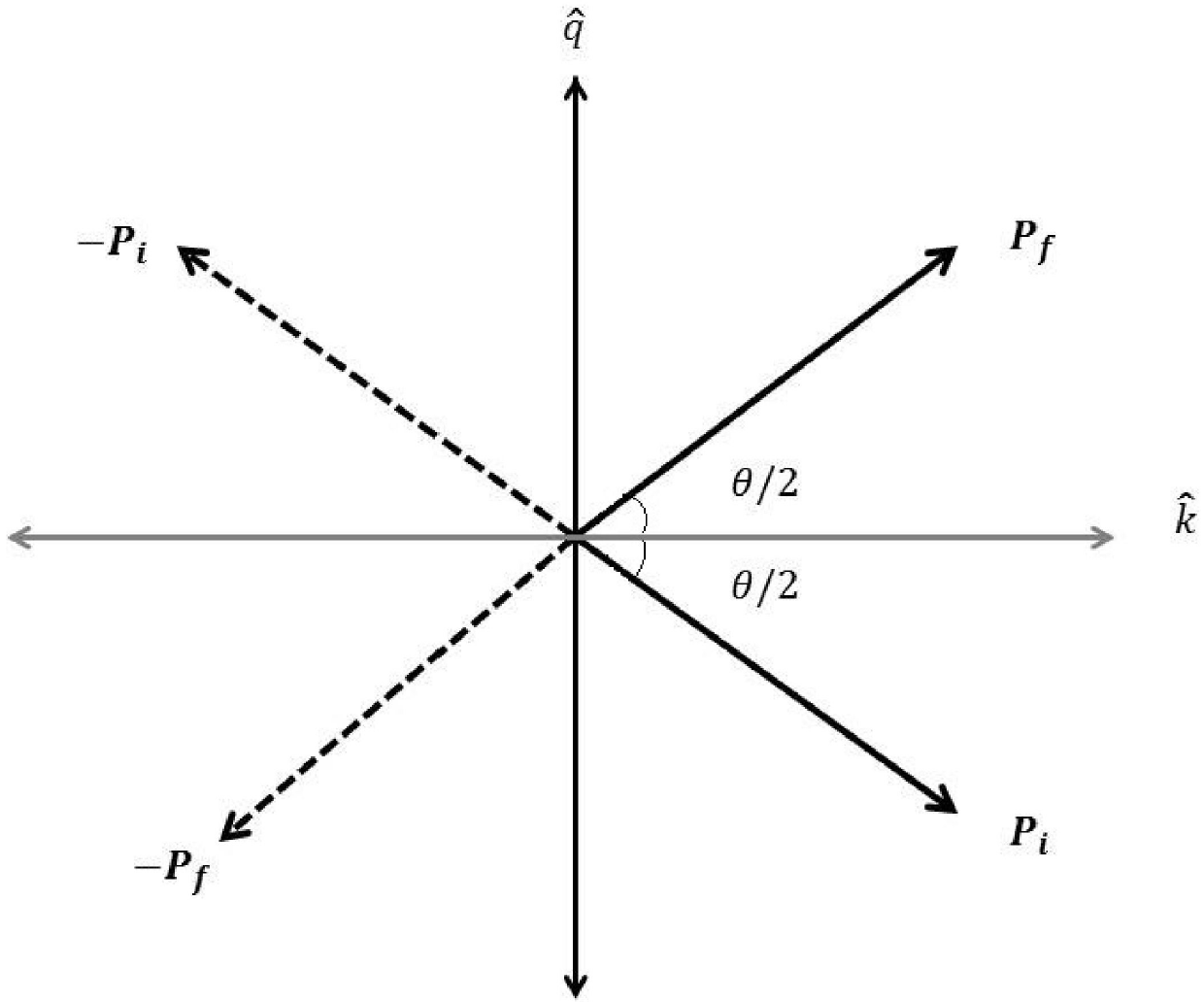
We now note that the two unit vectors;
k^=pf+pi|pf+pi|
along the total momentum and
q^=pf-pi|pf-pi|
along the momentum transfer are orthonormal; see Fig. 1. This is, of course, true for the scattering in any potential field.
Introducing a third unit vector l^=k^×q^ that is normal to the k^-q^ plane, we get a set of three mutually orthogonal unit vectors which we employ to define a new set of axes, see Fig. 2. To this end, we introduce the three operators Σk=Σ.k^; Σq=Σ.q^ and Σl=Σ.l^. Using the identity Σ.AΣ.B=A.B+iΣ.A×B we can immediately verify the following commutation and anti-commutation relations:
Σk,Σq=2iΣlΣl,Σk=2iΣq (8)Σq,Σl=2iΣk,.Σl,Σk=Σq,Σl=Σq,Σk=0 (9)
Thus, the consequences:
(Σk)2=(Σq)2=(Σl)2=I.
(10)
and,
iΣk=ΣqΣl, iΣq=ΣlΣk, iΣl=ΣkΣq
(11)
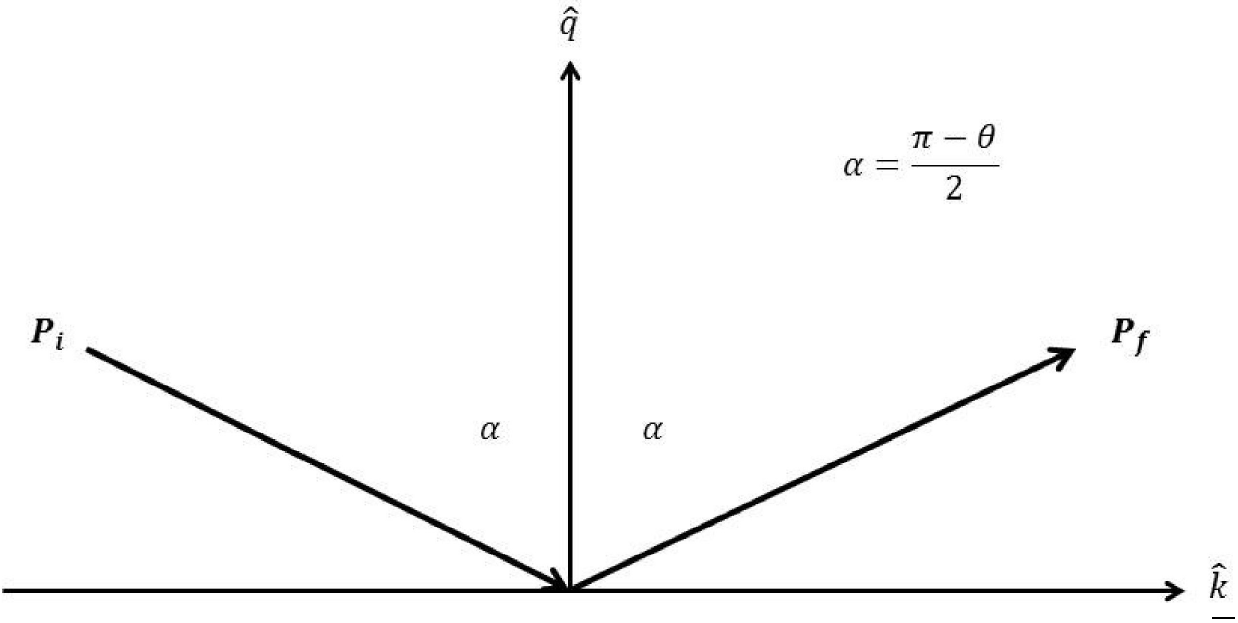
The above relations says that the newly introduced Σ matrices furnish a representation of the SU(2) algebra, and are generators of rotation in the spin space. We will now express all the spin operators and the SI in terms of these generators. We will thus, demonstrate that the description of the helicity-conserving first order transition in the spin space becomes more symmetric. To start with, express Σ.p^i and Σ.p^f in terms of Σk and Σq (see Fig. 2):
Σ.pi^=cosθ2Σk-sinθ2ΣqΣ.pf^=cosθ2Σk+sinθ2Σq
(12)
The symmetry in the above expression between the helicity operators of the initial and final particles - which goes with the symmetry in figure - is obvious. One can actually go further and check that - as the figure also suggests- Σ.pi^ and Σ.pf^ are related by a rotation about the l-axis:
Σ.pf^=U-1(l,θ)Σ.pi^U(l,θ)
(13)
The above equation makes explicit the intuitive picture that the spin of the incident particle gets rotated by an angle θ to remain aligned along the direction of the momentum.
3. The Transition in the k^-q^ Basis
In this section we will express the SI in terms of the newly introduced generators and investigate the interesting consequences of this. We will then write the scattering states in terms of the k^-basis and obtain an expression for the matrix element in terms of these basis. We first note the following major relations which can be easily proven using Eqs. (8)-(12):
Σ.pf^ΣkΣ.pi^=Σk (14)Σ.pf^ΣqΣ.pi^=-Σq (15)
Note how the above two equations go with the symmetry in Fig. 2. Now, from Fig. 3, we have the unit vector a^ appearing in the SI given as:
a^=a^.l^l^+a^.k^k^+a^.q^q^=Al^+Bk^+Cq^.
(16)
The spin interaction operator will then take the form:
γ5Σ.a^=Aγ5Σl+Bγ5Σk+Cγ5Σq
(17)
with A, B and C defined in Eq. (16) above. The transition matrix element, Eq. (7), upon employing the expansion given by Eq. (17) above can be further reduced. To do this, consider first the matrix element of Σq, namely ⟨pf^;±|γ5Σq|pi^;±⟩. This can be written (just by noting that the states are eigenstates of the initial and final helicity operators) as:
⟨pf^;±|γ5Σq|pi^;±⟩=⟨pf^;±|γ5Σ.pf^ΣqΣ.pi^|pi^;±⟩=-⟨pf^;±|γ5Σ.pf^ΣqΣ.pi^|pi^;±⟩
(18)
where we have used Eq. (15) to write the second line. Letting operators act on their eigenstates and noting that γ5 commutes with all the Σ's, we get
⟨pf^;±|γ5Σq|pi^;±⟩=-⟨pf^;±|γ5Σq|pi^;±⟩
(19)
with the obvious consequence:
⟨pf^;±|γ5Σq|pi^;±⟩=0
(20)
The Σq part of the SI does not contribute to the helicity-conserving transition. This should not be too surprising, as it is a guarantee of the gauge-invariance of the transition probability. Obviously, under a gauge transformation A(q)→A(q)+qf(q), with
f
(q) arbitrary. So, if the matrix element is to be gauge-invariant, which is indeed so, then the contribution of Σq should vanish. We now move to the Σl matrix element. This, again, can be expressed as:
⟨pf^;±|γ5Σl|pi^;±⟩=⟨pf^;±|γ5Σ.pf^ΣlΣ.pi^|pi^;±⟩
(21)
This can be reduced (see the appendix) to:
⟨pf^;±γ5Σ.pi^ΣlΣ.pi^pi^;±=±ipf^;±γ5-cosθ2Σq+sinθ2Σkpi^;±
(22)
The matrix element of the Σq component vanishes as we have demonstrated above, and we are left with the Σk contribution. Thus, putting every thing together we have the result:
⟨pf^;±γ5Σ.a^pi^;±=B±iAsinθ2⟨pf^;±|γ5Σk|pi; ^±
(23)
The transition is induced solely by γ5Σk, i.e the component of the spin interaction operator along the direction of the total momentum vector k!. To see what is special with this direction, look again at Fig. 2. The helicity-conserving transition is a transition that leaves the component of the spin along k^ invariant, while flipping the component along q^. This is what Eqs. (14) and (15) also say. Therefore, formulated in the k^-q^ basis, the conservation of helicity at first order scattering in a static magnetic field amounts to the conservation of the spin component along k^ in the transition and the flipping of the component along q^. This is just what happens to the momentum of a classical object; a ball say, as it bounces off a wall. The momentum along the wall is conserved, while that parallel to it flips. In our case, the “wall" is defined by the total momentum vector k, see Fig. 4. The transition, however, takes place in the spin space, and the relevant quantity is the orientation of the spin of the particle.
This picture can be enhanced by expanding the initial and final helicity states in terms of the eigenstates of Σk and Σq, which can be achieved by simple rotations about the l^-axis. We focus here on states with positive helicity; those with negative helicity can be obtained in exactly the same manner. Indeed, from Fig. 2, we can see that:
|pi^;+ =U I^, -θ2 |k^;+ = cosθ4 |k^;+ +sinθ4 |k^;- =U I^, -θ + π2 |q^;+ =cosθ + π4 |q^;+ +sinθ + π4 |q^;-
(24)
and,
|pf^;+ =U I^, θ2 |k^;+ = cosθ4 |k^;+ -sinθ4 |k^;- =U I^, θ - π2 |q^;+ =sinθ + π4 |q^;+ +cosθ + π4 |q^;-
(25)
Investigating the above equations it is obvious that
|⟨k^;±|pi^;+⟩|2=|⟨k^;±|pf^;+⟩|2
(26)
while,
|⟨q^;±|pi^;+⟩|2=|⟨q^;∓|pf^;+⟩|2
(27)
In fact, one can check directly that the SI interaction connects initial and final k^- states with the same helicity only, i.e.no flip, but different helicity q^- states. To see this, we consider the matrix elements ⟨k^;∓|γ5Σk|k^;±⟩ and ⟨q^;±|γ5Σk|q^;±⟩ and show that they both vanish. Consider the first one:
k^;∓γ5Σkk^;± = ± k^;∓γ5k^;± = k^;∓∓ Σkγ5± Σkk^;± = -k^;∓γ5k^;±
(28)
Thus,
k^;∓γ5Σkk^;± = ± k^;∓γ5k^;± = ∓k^;∓γ5k^;± =0
(29)
Similarly,
q^;±γ5Σkq^;± =q^;±Σqγ5ΣkΣqq^;± = -q^;±γ5Σkq^;±
where in the last line we noted that Σk and Σq anticommute in view of Eqs. (9). So, again:
⟨q^;±|γ5Σk|q^;±⟩=0
(30)
These results support our earlier arguments regarding the conservation of the k^ component and the flipping of the q^ component of the spin of the incident particle.
Finally, one can, by expanding the initial and final states in terms of the Σk eigenstates, thus eliminating any reference to these in the matrix element, express the matrix element totally in k^ variables and states. Starting from Eq. (23), we express the matrix element (see Eq. (24) and (25)) as:
Pf^;±γ5ΣkPi^;± =k^;±U-1I^, θ2γ5 × ΣkU I^, -θ2k^;±
(31)
One can easily check that
U-1l^,θ2γ5ΣkUl^,-θ2=γ5Σk
(32)
Combining this result with Eq. (23) we get
Pf^;±γ5 Σ.a^Pi^;± = B ±i Asinθ2 × k^;±γ5 Σkk^;±
(33)
Acting with Σk on its eigenstates, we get the result:
Pf^;±γ5 Σ.a^Pi^;± = ±B ±i Asinθ2 × k^;±γ5k^;±
(34)
In the above equation, the only reference to the initial and final states is through the kinematical/geometrical factors A and B. So, to calculate the transition matrix element for any vector potential, just find these factors - which is a trivial task- and plug them into the above expression. Things can be even further simplified if we use the explicit forms of the spinors:
|k^;±⟩=N'χ±σ.k0E+mχ±
(35)
where χ± are eigenstates of σ.k0 with eigenvalues ±1, and k0=pk^0 is a vector along k^0 with p being the conserved magnitude of the initial and the final momenta. Plugging this expression into Eq. (34) and using
γ5=0II0,
we have:
Pf^;±γ5 Σ.a^Pi^;± = ±B ±i Asinθ2 × 2N'2pE +m
(36)
This is just a “plug and play" formula, where one just fixes the geometrical factors A and B for the specific vector potential present, and then gets the spin sector of the matrix element immediately. The following two examples illustrate this explicitly.
4. Examples
In this section we consider two concrete examples of vector potentials whose field configurations conserve helicity, and we bring the first order transition matrix elements of Dirac particles in these potentials to the form given by Eq. (34). Consider first the Ahronov-Bohm (AB) potential 3 which gives rise to a δ-function mgnetic field extended along the z-axis. This vector potential is given as:
A(r)=Φ2π-yx^+xy^x2+y2=Φ2πρϵ^φ,
(37)
where ρ=x2+y2, ϵ^φ is the unit vector in the φ-direction, and Φ is the flux through the AB tube. Since the magnetic field is along the z-axis; the z-component of the incident momentum doe not change during the scattering process. Therefore, we consider normal scattering, i.e. take the incident, and consequently, the outgoing momenta to be in the x - y plane. In such a geometry, l^ is just z^. Pluggingb this vector potential into Eq. (7), we get:
Sfi1= -2πeN2δEf-Eiuf†pf, sf × -eΦα1q2-α2q1q2 ui pi, si
(38)
So,
A(q)=-Φq2x^-q1y^q2=-Φqa^(q)
(39)
with a^(q) given as
a^(q)=q2x^-q1y^q
(40)
For the purpose of applying the formula (34), we need to find the geometrical factors A and B. Obviously, A = 0. As for B, we note that we can without any loss of generality, take the incident momentum to be along the x-axis; pi=px^ so that
pf=pcosθ2x^+sinθ2y^.
Straight forward algebra shows that with such a choice of the incident momentum, we get a^(q)=k^, so that γ5Σ.a^=γ5Σ.k^, meaning that B = 1. The matrix element for the AB potential then becomes 4:
M= Pf^;±γ5 Σ.a^Pi^;± = Pf^;±γ5 Σ.k^Pi^;± = ± k^;±γ5k^;±
(41)
We can even move to calculate the scattering cross section. The unpolarized scattering cross section of a Dirac particle in the AB field is given as 5,6,7:
dσdθ=e2Φ22πp3sin2θ212∑si,sf=±|⟨pf^;sf|γ5Σ.a^|pi^;si⟩|2
(42)
where the summation is over the initial and final particles’ helicities. As a consequence of Eqs. (41) we have
⟨pf^;-|γ5Σ.a^|pi^;-⟩=-⟨k^;+|γ5|k^;+⟩=-⟨pf^;+|γ5Σ.a^|pi^;+⟩.
So, using Eq. (33), and taking the normalization constant
N'=E+m4m
we get
dσdθ=e2Φ28πp sin2θ2
(43)
which is the well-known AB scatttering cross section of a Dirac particle at first order 5.
The second example is the vector potential of a magnetic dipole, and is less symmetric as the resulting field is not, contrary to the AB one, axial. The vector potential of the dipole is given by 8
A(r)=μ×rr3
(44)
where μ is the magnetic moment. The Fourier transform of the above vector potential is (up to a numerical factor) A(q)=(μ×q/q2). Thus, the first order matrix element reads
Sfi1= -2πeN2 | 1q2 δEf-Eiuf†pf, sf × γ5Σ.μ × qμ × q ui pi, si
(45)
Therefore
a^=μ×q|μ×q|.
The kinematical factors of Eq. (33) are just
A=l^.μ×q|μ×q|
and
B=k^.μ×q|μ×q|.
which are straight forward to calculate; just specify μ and p
i. Therefore, the transition matrix element reads now:
Sfi1= ∓2πeN2 | 1q2 δEf-Ei × k^.μ × qμ × q±il^.μ × qμ × qsinθ2 × ⟨k^;±|γ5|k^;±⟩
(46)
The cross section can be calculated straight forwardly from the above amplitude.
5. Conclusions
The spin interaction in the first order S-matrix of a Dirac particle in a static magnetic field was investigated. Noting that the total momentum vector k = p
f
+ p
i and the momentum transfer vector q = p
f
- p
i are always perpendicular, we suggested that the three unit vectors; k^, q^ and l^≡k^×q^ defined an “intrinsic" coordinate system, where the transition, and particularly, the conservation of helicity, could be described in an alternative, more symmetric formalism. The three generators Σk≡Σ.k^, Σq≡Σ.q^, and Σl≡Σ.l^ were shown to close the SU(2) algebra. When the spin interaction operator γ5Σ.a^ was written in terms of these generators, we have been able to reduce the transition in the spin space to an expression proportional to the matrix element of the operator γ5Σk.
Expressing Σ.pi^ and Σ.pf^ and their eigenstates in terms of Σk, Σq, and their eigenstates, we have demonstrated that the conservation of helicity can be formulated as the invariance of the k^ component of the spin of the particle and the flipping of its q^ component. An intuitive physical picture of the transition, similar to that of a ball bouncing off a wall was suggested. The scattering matrix element was written, for any static field configuration, as the matrix element of the γ5Σk in Σk basis, multiplied by kinematical/geometrical factors which carry the only reference to the initial and final momenta.
References
1. M. Jacob and G.C. Wick, Ann. Phys. 7 (1959) 404.
[ Links ]
2. J.J. Sakurai, Advanced Quantum Mechanics (Addison-Wesley, Massachusettes, 1967).
[ Links ]
3. Y. Aharonov and D. Bohm, Phys. Rev. 115 (1959) 485.
[ Links ]
4. A. Albeed and M.S. Shikakhwa, Int. J. Theor. Phys. 47 (2008) 2748.
[ Links ]
5. F. Vera and I. Schmidt, Phys. Rev. D 42 (1990) 3591.
[ Links ]
6. M.S. Shikakhwa and N.K. Pak, Phys. Rev. D 67 (2003) 105019.
[ Links ]
7. M. Boz and N.K. Pak , Phys. Rev. D 62 (2000) 045022.
[ Links ]
8. J.D. Jackson, Classical Electrodynamics (second edition, John Wiley and Sons, 1975).
[ Links ]
Appendix
A.
We show here how to derive Eqs. (22) in the text. We start with
⟨pf^;±|γ5Σl|pi^;±⟩=⟨pf^;±|γ5Σ.pf^ΣlΣ.pi^|pi^;±⟩
(A.1)
Look at:
Σ.pf^ Σl Σ.pi^ | pi^; ± = Σ.pf^ Σl × cosθ2 Σk -sinθ2 Σq | pi^; ±
(A.2)
Using Eqs. (11), this can be written as:
Σ.pf^ Σl Σ.pi^ | pi^; ± =iΣ.pf^ × cosθ2 Σq +sinθ2 Σk | pi^; ±
(A.3)
Eqs. (14) and (15) allow us to re-introduce Σ.pi^ and thus bring this into the form
Σ.pf^ Σl Σ.pi^ | pi^; ± =i-cosθ2 ΣqΣ.pi^+sinθ2 ΣkΣ.pi^ | pi^; ±
(A.4)
Allowing the operator Σ.pi^ to act on its eigenstates, we get:
Σ.pf^ Σl Σ.pi^ | pi^; ± =±i-cosθ2 Σq+sinθ2 Σk | pi^; ±
(A.5)
Our result, now, follows immediately;
⟨pf^;±|γ5 Σl|pi^;±⟩=±i ⟨pf^;±|γ5 × -cosθ2 Σq+sinθ2 Σk | pi^; ±
(A.6)


 nueva página del texto (beta)
 Inglés (pdf)
 Artículo en XML
 Referencias del artículo
 Enviar artículo por email
 Citado por SciELO
  Similares en
SciELO
Similares en
SciELO 
 Permalink