SciELO - Scientific Electronic Library Online

 
vol.63 issue5On the decay of an accelerated protonStable bound states of N’s, Λ ’s and Ξ ’s author indexsubject indexsearch form
Home Pagealphabetic serial listing  

Services on Demand

Journal

Article

Indicators

Related links

  • Have no similar articlesSimilars in SciELO

Share


Revista mexicana de física

Print version ISSN 0035-001X

Rev. mex. fis. vol.63 n.5 México Sep./Oct. 2017


Research

Electromagnetic transmittance in alternating material-metamaterial layered structures

V.H. Carrera-Escobedoa 

H.C. Rosua  * 

1Instituto Potosino de Investigación Científica y Tecnológica, Camino a la presa San José 2055, Col. Lomas 4a Sección, 78216 San Luis Potosí, S.L.P., México.


Abstract

Using the transfer matrix method we examine the parametric behavior of the transmittance of TE and TM electromagnetic plane waves propagating in frequency range which are far from the absorption bands of a periodic multilayered system. We focus on the dependence of the transmittance on the frequency and angle of incidence of the electromagnetic wave for the case in which the periodic structure comprises alternating material-metamaterial layers of various permittivities and permeabilities. A specific example of high transmittance at any angle of incidence in the visible region of the spectrum is identified.

Keywords: Transfer matrix method; transmittance; metamaterial; multilayer; periodic

Resumen

Usando el método de la matriz de transferencia examinamos la dependencia paramétrica de la transmitancia de las ondas planas electromagnéticas TE y TM en rangos de frecuencia lejanos de las bandas de absorción de un sistema multicapas periodico. Nos enfocamos en la dependencia de la transmitancia de la frecuencia y el ángulo de incidencia de la onda electromagnética para el caso en el cual la estructura periodica contiene una alternancia de capas de material y metamaterial de varias permitividades y permeabilidades. Un ejemplo especifico de transmitancia alta para cualquier ángulo es identificado en la región del espectro visible.

Palabras clave: Método de la matriz de transferencia; transmitancia; metamaterial; multicapa; periodico

PACS: 02.30.Hq; 11.30.Pb

1. Introduction

Studies of planar multilayer structures with alternating material and metamaterial layers are motivated by the known common feature of planar periodic systems to generate transparency bands. Some time ago, Banerjee et al1 calculated the intensity of the electromagnetic fields that propagate through an array of periodically alternating positive index media (PIM) and negative index media (NIM). However, they do not present their results in terms of either the angle of incidence or the frequency of the plane wave, which are the important parameters when one is interested in the directional and frequency selectivities of such structures. They display the field intensity along the direction of propagation and compare the transfer matrix method to the finite element method concluding that the transfer matrix method provides the same results as the latter. Their results motivated us to use the transfer matrix method with the main goal of studying the effect of both the angle of incidence and frequency of the propagating plane wave on the transmittance spectrum. We compute the values of the transmittance for different values of ϵ and μ of the alternating material-metamaterial layers and search for those values that provide wide windows of transmittance for some regions of frequency as well as the complementary transmittance gaps that may be useful for making frequency filters 2.

2. The transfer matrix method

2.1. Waves at an interface

To develop the TMM we must first know how the electromagnetic waves behave at the interface between two dielectrics. For plane waves at an interface, the electric and magnetic fields are given by

E=E0eikr-ωt (1)

H=H0eikr-ωt (2)

respectively. The two media separated by the interface will be characterized by permittivities ϵ1, ϵ2 and permeabilities μ1, μ2, and the geometry of the wave vectors at the interface is illustrated in Fig. (1). In this figure, we assume that the wave is propagating along the z-axis and the wavevector has two components, k=(kx,0,kz).

Figure 1. Electromagnetic wave vectors at the interface between two different media. 

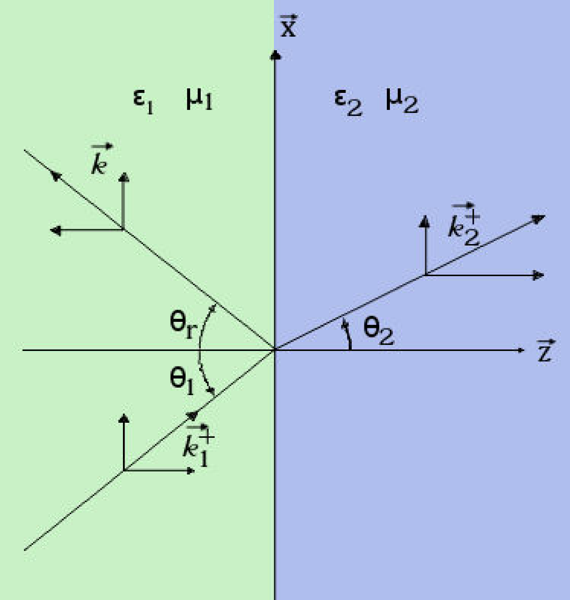
Because the condition of continuity of the tangential components of both the electric and magnetic fields

E1t=E2t, H1t=H2t (3)

must be satisfied for any point of the interface, the tangential components of k have to be equal

k1x=k2x=kx, (4)

while the dispersion relation n2ω2/c2=k2 as written for the two media leads to

n12ω2c2=k12=kx2+k1z2,n1=μ1ϵ1,    (5)n22ω2c2=k22=kx2+k2z2,n2=μ2ϵ2.   (6)

If k x and k z are real, we can define the angles of incidence and refraction as

tanθ1=kxk1z (7)

and

tanθ2=kxk2z, (8)

respectively. From Eq. (4), we can see that

kx=k1sinθ1=k2sinθ2 (9)

and if we apply the dispersion relationship, we obtain

kx=n1ωcsinθ1=n2ωcsinθ2. (10)

If we now take the ratio of the last two equations we obtain Snell’s law

sinθ1sinθ2=n2n1. (11)

Considering the case of the TE polarization (s-type polarization), then E is parallel to the interface, i.e., we have

E=(0,E,0) (12)

and

H=(Hx,0,Hz). (13)

We also have the boundary condition that says that the component of the electric field which is parallel to the interface is the same on both sides of the interfaces

E1++E1-=E2++E2-, (14)

which holds for the magnetic field

H1x++H1x-=H2x++H2x- (15)

as well as.

Using Maxwell’s equation

k×E=+μωcH, (16)

in Eq. (15), we obtain

μ1ωcH1x+=-k1zE1+,        (17)μ1ωcH1x-=k1zE1-.           (18)

Inserting (17) in (15) leads to

-k1zcμ1ωE1++k1zcμ1ωE1-=-k2zcμ2ωE2++k2zcμ2ωE2-. (19)

Now we can write Equations (19) and (14) in matrix form

(11-k1zμ1k1zμ1)(E1+E1-)=(11-k2zμ2k2zμ2)(E2+E2-) (20)

or

(E2+E2-)=M(s)(E1+E1-) (21)

where the transfer matrix of the interface

M(s)=12(1+μ2k1zμ1k2z1-μ2k1zμ1k2z1-μ2k1zμ1k2z1+μ2k1zμ1k2z) (22)

is introduced.

By a similar procedure, we can obtain the transfer matrix for the case of the TM polarization (p-type polarization)

(E2+E2-)=MpE1+E1-                                                             (23)M(p)=121+ϵ2k1zϵ1k2z1-ϵ2k1zϵ1k2z1-ϵ2k1zϵ1k2z1+ϵ2k1zϵ1k2z.                              (24)

For materials with only real dielectric constants we can express the wave vectors as

k1z=k1cosθ1            and           k2zcosθ2 (25)

so the transfer matrices for the TE and TM cases are written as

M(s  or  p)=12(1+z21cosθ1cosθ21-z21cosθ1cosθ21-z21cosθ1cosθ21+z21cosθ1cosθ2) (26)

where z21=μ2k1/μ1k2 for the s-polarization and z21=ϵ2k1/ϵ1k2 for the p-polarization.

2.2. The transfer matrix for a slab

For a set of interfaces, the systems behaves as a slab (sandwich of media). A simple example is given in Fig. (2).

Figure 2. Illustration of wave propagation through a slab composed of three different media. 

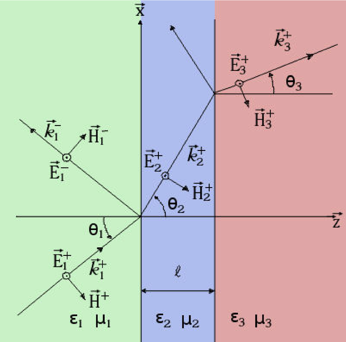
For such systems, it is enough to apply the composition law for transfer matrices 3. In this way, the relationship of the coefficients of entry and exit is given by

(E3+E3-)=M12(eik2zl00e-ik2zl)×M23(E1+E1-), (27)

where l is the length of the slab in the direction of propagation.

From the last equation, one can obtain the transfer matrix for the slab as

Mslabs=M12(eik2zl00e-ik2zl)M23, (28)

which can be used for the generalization to the multilayer case.

2.3. Wave propagation through a multilayered system

The next step is to consider a multilayered system as illustrated in Fig. (3).

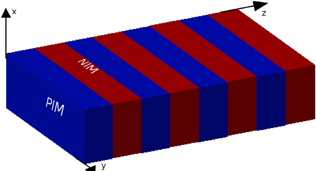
Figure 3. A system formed by two types of slabs. The first one is a PIM (blue) labeled as A in the text, and the second is a NIM (red) labeled as B in the text. 

For a system of this class, the transfer matrix is obtained by applying the composition law again. In this way, we have an interface matrix M i,i+1 for every interface and a propagation matrix of the form

P=(eik2zl00e-ik2zl) (29)

for every slab in which the electromagnetic wave propagates. In this manner, for a ten multilayer slab system (5 A and 5 B layers) the transfer matrix is written as

M=M0APAMABPBMBA4PAMABPBMB0 (30)

where M 0X is the interface matrix between air and medium X, P X is the propagation matrix of medium X, and M XY is the interface matrix between medium X and medium Y. The M and M XY matrices are transfer matrices for the s-polarization or the p-polarization, depending on the nature of the incident wave.

Once the transfer matrix for the multilayered system has been defined, one can proceed with the calculation of the transmission amplitude based on its definition for the case of electromagnetic waves given by 3

t=detMM22, (31)

where det M stands for the determinant of M, and the transmittance as its square modulus

T=|t|2. (32)

3. Numerical simulations

The computation of the transmittance is performed by using a simple python code 4. The system which we model has up to ten slabs, alternating a PIM with a NIM. The PIM is characterized by μ+ and ϵ+, while the NIM by μ- and ϵ-. The frequency of the incident wave is in c/(lϵ0) units, where the chosen numerical value for l is 1.0 μm, and the angle of incidence θ goes from -π/2<θ<π/2 which we normalize to θ0=π/2 in the figures. The plots of the transmittance versus frequency are obtained for an angle of incidence of π/3 radians. The range of frequencies goes from 300 THz to 1200 THz, which entails the frequency band of the visible light (430-770 THz). In the units of the plots, the band of frequencies of the visible light is [1.4-2.5] and is indicated by two horizontal black solid lines in the contour figures.

3.1. The effect of the number of layers

We begin by analyzing the effect of the number of layers upon the transmission spectrum. With this task in mind, we vary the number of periods “AB” crossed by the propagating wave using the values of the parameters given in Table I, where the parameters ϵ0 and μ0 correspond to the respective values for the relative permittivity and permittivity of the medium (usually air) in front and at the end of the “AB” multilayer structure. We call the “AB” period a block. In Fig. (7), the number of blocks is increased from two to five, (in terms of interfaces, from five to eleven), and each panel is labeled by the corresponding number of blocks. The regions of high transmittance show up as three symmetrical bubbles. Upon increasing the number of blocks in the system, one can see that the number of peaks inside each of the bubbles increases. The number of peaks, npeaks, is equal to twice the number of blocks, n b , minus one, npeaks=2nb-1. This might be seen alike to the case of quantum systems if the number of quantum wells is put in correspondence with the number of peaks in the transmittance. One can also see that when the number of blocks increases the transmittance between the bubbles of high transmittance becomes smaller. This is a consequence of the change in the transmittance values that one can see in Fig. (4), where we can also notice that the transmittance bands get wider as the number of blocks increases. Moreover, in Fig. (7), we can see that we have a bubble of high transmittance inside the limits of the visible frequencies (black horizontal lines), which could be useful for camouflage purposes. In addition, as we increase the number of blocks, this high transmittance region entails a wider range of angular values. On the other hand, if we increase the number of blocks enough the simulation ends up in a completely opaque material with zero transmittance, as expected.

Table I. The values of the permeabilities and permittivities of the AB slabs used for the case of a variable number of blocks. 

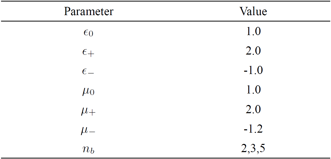
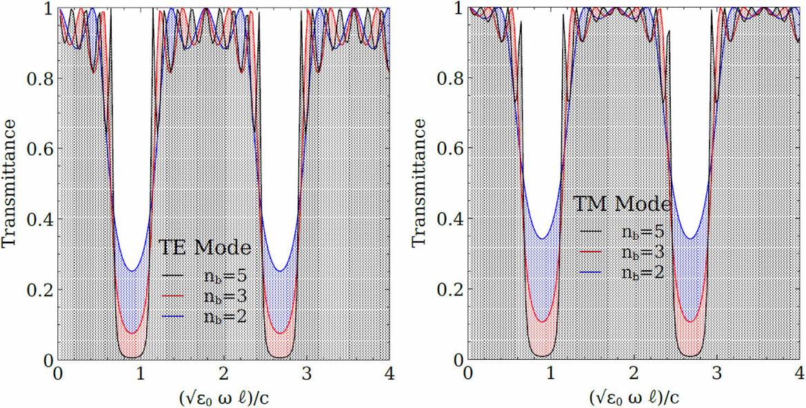
Figure 4. Plots corresponding to the case of variable number of blocks. Left panel: the TE mode. Right panel: the TM mode. In these graphs we can see that the valleys of the transmittance get deeper as we increase the number of blocks. This is congruent with the formation of transmission bands in the case of superlattices. 

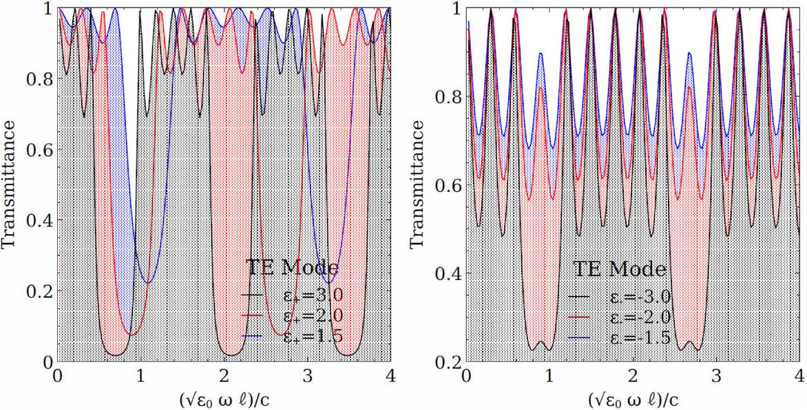
Figure 5. Plots corresponding to the case of fixed angle of incidence θ=π3. The left panel corresponds to the case of variable ϵ+ and the right panel corresponds to the case of variable ϵ-. In these graphs, we can see the shifting of the peaks in transmittance only for the case with increasing ϵ+

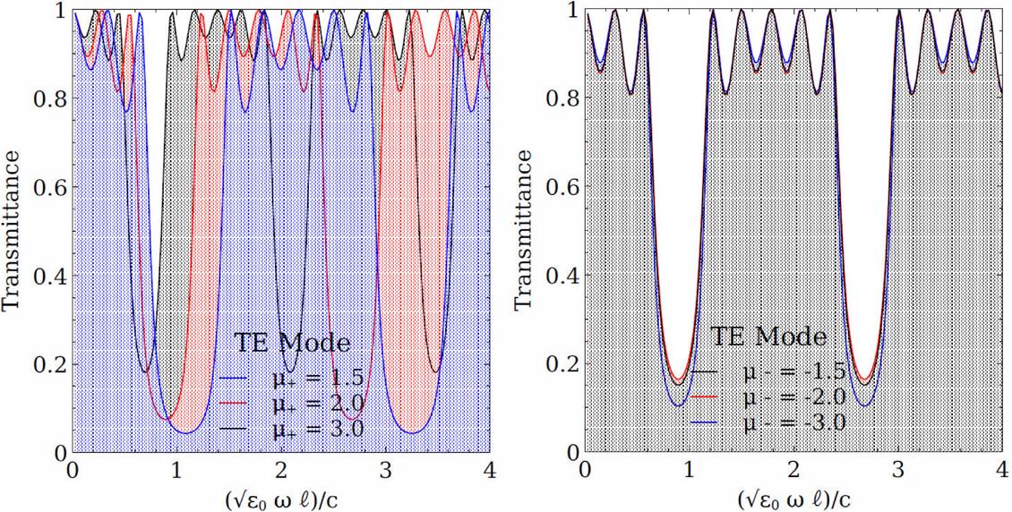
Figure 6. Plots corresponding to the case of fixed angle of incidence θ=π3. Left panel: case of variable μ+. Right panel: case of variable μ-. One can see that the shifting of the peaks in transmittance occurs only upon increasing μ+ (left panel) and there is no shifting effect when μ- is increased (right panel). 

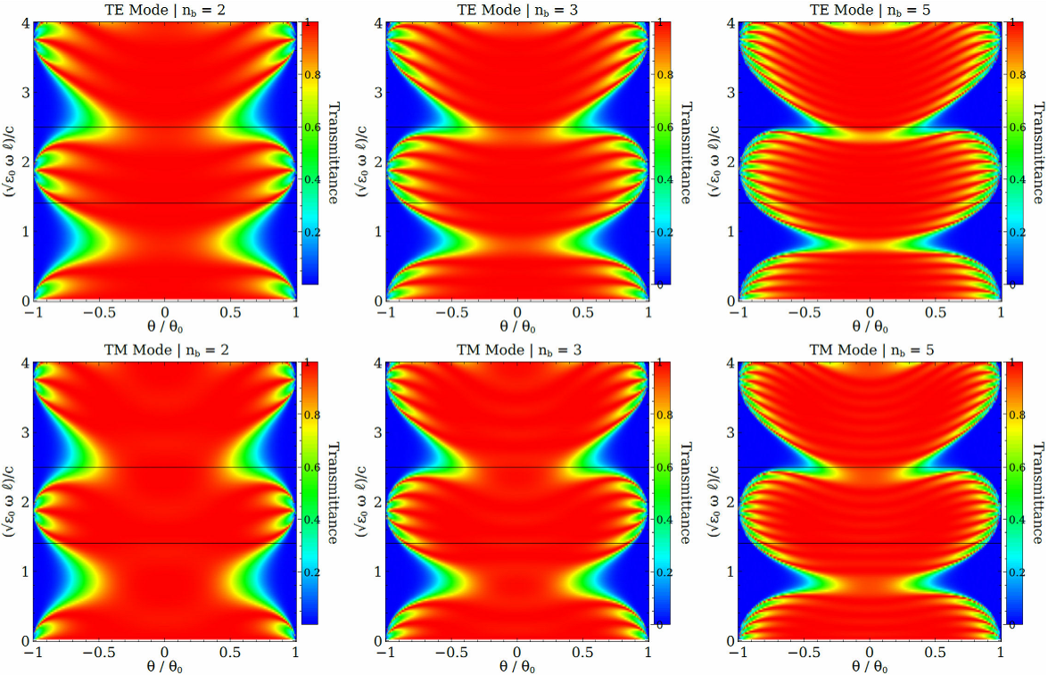
Figure 7. Contour plots. The top row correspond to the TE mode (s-polarization) while the bottom row correspond to the TM mode (p-polarization). The number of blocks takes the values n b = 2, 3, 5. The x-axis corresponds to the angle of incidence, the y-axis to the frequency of incidence in ϵ0lc units, and the color bar correspond to transmittance. The black horizontal lines indicate the limits of the frequencies of the visible range. 

3.2. The effect of ϵ+ and ϵ-

Knowing that the number of blocks generates a series of transmittance bands, one naturally may ask if there is a way to control the width of these bands by means of the electric permittivities of the slabs. The values of the parameters that we use for this computation are given in Table II.

Table II. The values of the permeability and permittivity used when the number of blocks is kept fixed. 

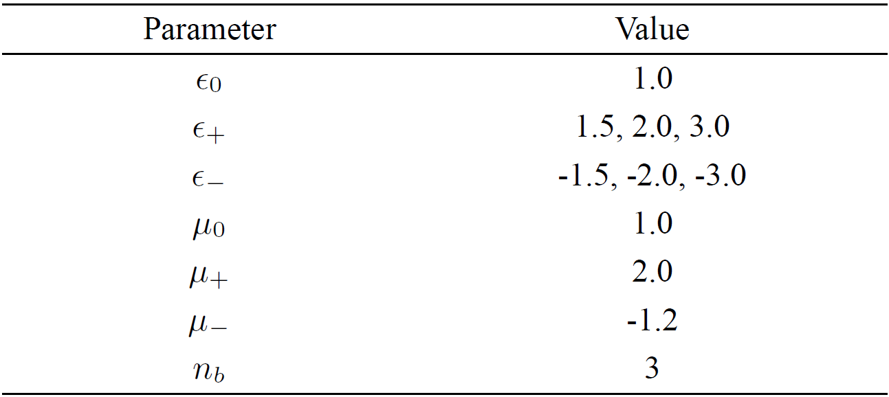
The results are presented in Fig. (8). We can see that the effect of increasing ϵ+ while keeping ϵ- fixed at -1.0, is to tighten the bubbles of high transmittance, and the magnitude of this effect is proportional to the increase in ϵ+. When ϵ+ is high enough, the bubbles lose the connection between them and become independent ovals. For this case, we see that the effect is similar for both the TE and TM modes, but for the TM mode the bubbles are more separated and there appears a series of smaller bubbles of high transmittance. Moreover, for both types of modes there is a shift to lower frequencies of these bubbles of high transmittance. This can be seen in the left panel of Fig. (5).

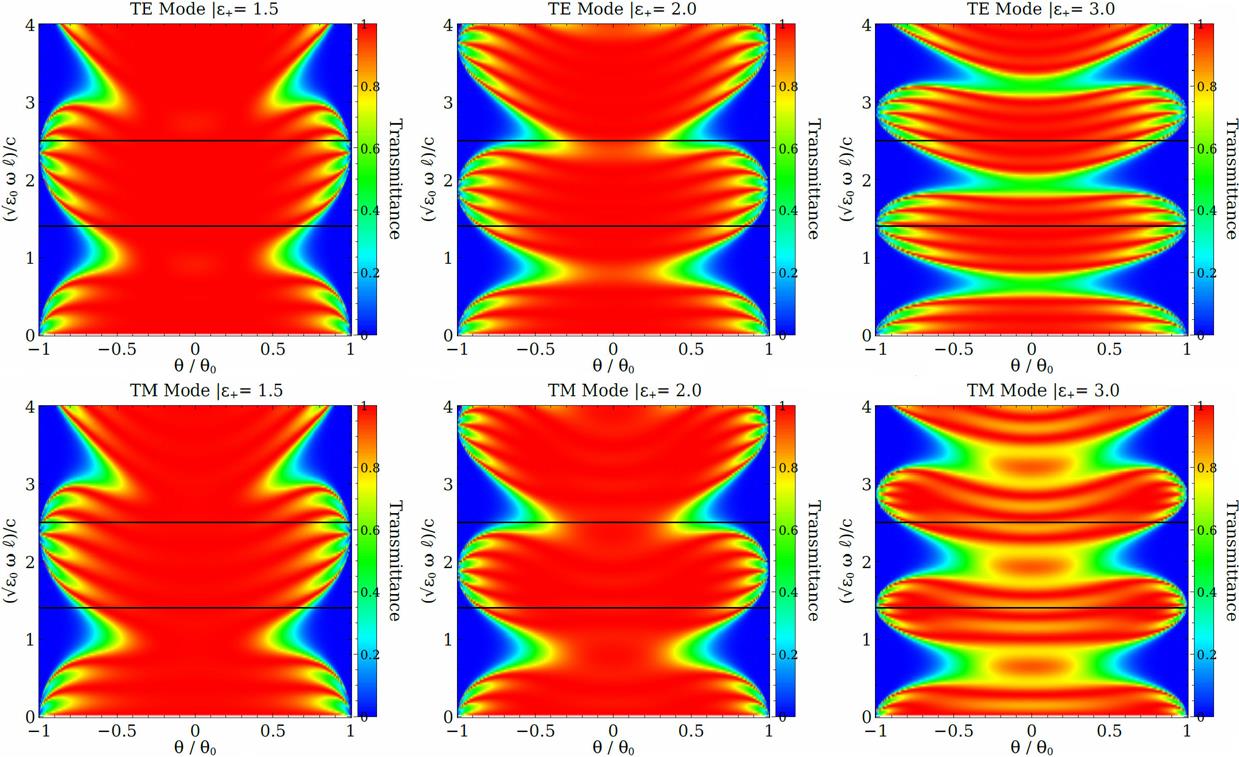
Figure 8. Contour plots. The top row correspond to the TE mode while the bottom row correspond to the TM mode. The positive permeability takes values ϵ+=1.5, 2, 3 while ϵ- is fixed at -1.0. 

On the other hand, if we increase the value of |ϵ-| while keeping ϵ+ fixed at 2.0 we can see from Fig. (9) that the bubbles of high transmittance are absent and in their place a wide band with horizontal spikes occurs. Therefore, we conclude that the occurrence of bubbles depend on the chosen values of ϵ+. When ϵ- increases, we can see that the wide band is fragmented in three sections, and the separation between sections is proportional to the increment in |ϵ-|. In this case, there is no shift to lower frequencies. This fact can be observed in the right panel of Fig. (5). The effect is similar for both TE and TM modes, but in the TM case the decrease in transmittance is less but in a wider range of frequencies.

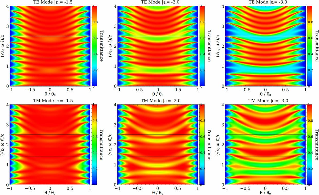
Figure 9. Contour plots. The top row correspond to the TE mode while the bottom row correspond to the TM mode. The positive permeability takes values ϵ- =1.5, 2, 3 while ϵ+ is fixed at 2.0. 

In general, we can say that the value of ϵ+ determines the form of the transmittance bands and the frequency range where they occur. On the other hand, the value of ϵ- determines the width of the horizontal transmittance spikes.

3.3. The effect of μ+ and μ-

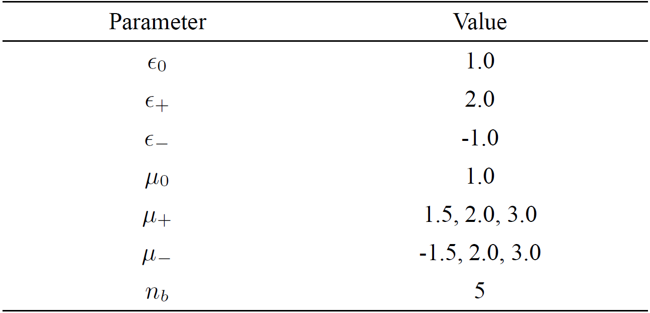
We move now to the study of the effects of increasing the values of the permeabilities of the system. For this task, we use the values from Table III for the parameters under control.

Table III. The parameters used when the μ values are changed. 

From Fig. (6), we see that if we increase the magnitude of μ+ the bubbles of high transmittance have a shift to lower frequencies which is proportional to the magnitude of μ+. Unlike the case of varying ϵ+, we see that the bubbles remain connected, and as the value of μ+ increases the contact area between bubbles increases as well as. This is opposite to the case of varying ϵ+ and occurs for both the TE and TM modes.

From the left panel of Fig. (11), we can appreciate easily a shifting effect to lower frequencies. Also, and even more interesting, we see that if we increase the value of μ+ the valleys (regions of low transmittance) become less apparent. Thus, increasing μ+ has the effect of rising the valleys of transmittance diminishing the relative borders of the transmittance bands.

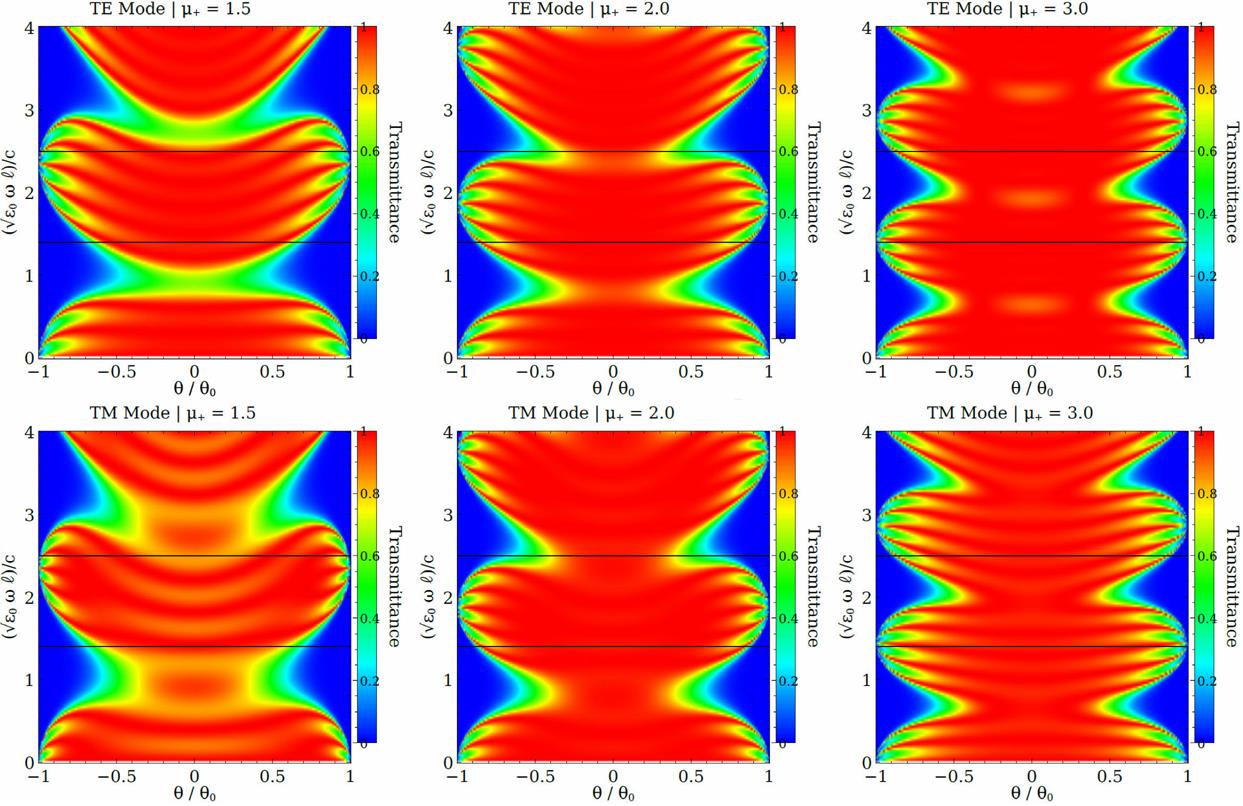
Figure 10. Contour plots. The top row correspond to the TE mode while the bottom row correspond to the TM mode. μ- is fixed at -1.2. 

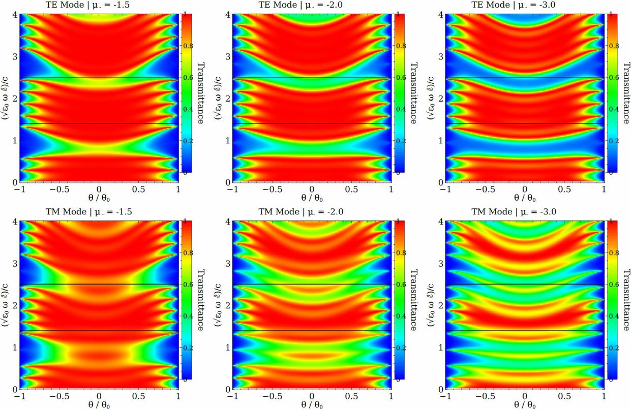
Figure 11. Contour plots. The top row correspond to the TE mode while the bottom row correspond to the TM mode. μ+ is fixed at 1.2. 

In the case of increasing the values of |μ-|, Fig. (11) shows that the main effect is to diminish the transmittance between the three regions of high transmittance. This effect is also visible on both the TE and TM modes. However, in this case, we notice that there is no shifting effect, which can be seen easily from the right panel of Fig. (6).

In addition, Figs. (7)-(11) show that the regions of high transmittance do not vary with the angle of incidence, which may be related to the independence of the polarization angle of the incident wave as also reported in 5. Considering that the reflectance and transmittance are complementary properties, our findings regarding the transmittance spectrum seem to be in agreement with those reported in 6 for an Ag-TiO2 multilayer system, which is the standard multilayer candidate with high transmittance in the visible region.

4. Conclusion

We have obtained the transmission properties of a multilayered structure of alternating positive index media and negative index media using the TMM. We have sought for profiles of high transmittance at any angle of incidence in the visible region of the spectrum. In this respect, our results suggest a system with the properties displayed in Fig. (7), i.e., with ϵ+=2.0,ϵ-=-1.0,μ+=2.0, and μ-=-1.2, for the case of five blocks, n b = 5, which present an almost uniform region of high transmittance in the visible part of the electromagnetic spectrum.

In addition, we have studied the manner in which the permeability and permittivity parameters affect the transmission properties in an alternation of material and metamaterial. We have observed that positive permeabilities may have the effect of reversing the appearance of the transmission bands that one may see in multilayered structures. On the contrary, positive permittivities have the effect of making the transmittance bands more pronounced. Somewhat surprisingly, the negative values of the electromagnetic material parameters do not have relevant effects in these settings.

The results obtained in this paper are valid far from the absorption bands of the multilayer structure to avoid numerical instability problems which are known to occur when the absorption is included 7. However, the results we report for the visible region may still remain valid for some metamaterials, such as the hyperbolic ones, for which the absorption bands lie in the ultraviolet region 8.

Acknowledgments

The first author acknowledges the financial support of CONACyT through a doctoral fellowship at IPICyT.

References

1. P.P. Banerjee, H. Li, R. Aylo, and G. Nehmetallah, Proc. SPIE 8093 (2011) 3387-3389. [ Links ]

2. L. Solymar and E. Shamonina, “Waves in Metamaterials” (Oxford University Press, 2009). [ Links ]

3. P. Markos and C.M. Soukoulis, “Wave propagation from electrons to photonic crystals and left-handed materials” (Princeton University Press, 2008). [ Links ]

4. Python Software Foundation. Python Language Reference, version 2.7. Available at http://www.python.org. [ Links ]

5. B.-X. Wang, Plasmonics 12 (2017) 95-102. [ Links ]

6. P. Shekhar, J. Atkinson, and Z. Jacob, Nano Convergence 1 (2014) 14. [ Links ]

7. W.-J. Hsueh and J.-C. Lin, J. Opt. Soc. Am. 24 (2007) 825-830. [ Links ]

8. T. Tumkur, Y. Barnakov, S.T. Kee, M.A. Noginov, and V. Liberman J. Appl. Phys. 117 (2015) 103104. [ Links ]

Received: March 27, 2017; Accepted: May 29, 2017

Creative Commons License This is an open-access article distributed under the terms of the Creative Commons Attribution License