


 nueva página del texto (beta)
 Inglés (pdf)
 Artículo en XML
 Referencias del artículo
 Enviar artículo por email
 Citado por SciELO
  Similares en
SciELO
Similares en
SciELO 
 Permalink
PACS: 47.32 cb; 47.27 ek; 47.27 De
1. Introduction
Counter-rotating vortex pairs (known as “dipoles”) are observed in flows exiting channels. Examples of these structures have been reported, for example, in laboratory experiments for tidal starting-jet vortices 9, in geophysical systems such as the Venetian lagoon 6, and in gulfs in northern Patagonia 1. Depending on the tide stage, the flow rate can be positive (seaward flow) or negative (inward flow). Wells-van Heijst 14 modeled the generation and evolution of a dipole in which the flow is the sum of a linear source (or sink) and two vortices of equal strength and opposite sign. According to this model, whether the vortices escape or remain near the channel depends on the Strouhal number S, which is defined as
where H1 is the channel width, U is the maximum velocity of the fluid at the channel output, and T is the driving period. For S < 0.13 the circulation and the size of the vortices grow at the beginning of each cycle and, given sufficient time, dipoles escape because of their self-induced velocity. Conversely, for S < 0.13, dipoles are sucked inward during the stage of negative flow rate.
Although the Wells-van Heijst model (hereafter referred to as the W-H model) correctly describes the conditions under which dipoles escape or are retained, it fails to reproduce features such as the small-S dipole properties. Otherwise, the model is not intended to account the persistence of dipoles for more than one period, or the interaction between two consecutive dipoles. The interaction between consecutive vortices leads to phenomena such as the coalescence of vortices or the reduction of its translational speed. Such vortex interactions and vortex mergers have been studied before in various external flows both numerically and experimentally 2,10,13.
A previous work 8 has shown that, for small Strouhal numbers, two or more dipoles may coexist without appreciably interaction. However, the main interest of the present work is to study the coexistence of dipoles and their interaction. To achieve this objective, we present results of numerical simulations with the Strouhal numbers between 0.05 and 0.1.
This paper is organized as follows: Section 2 describes the geometry of the system, the equations governing the flow, and the methodology. We introduce two dimensionless parameters and the quantities calculated with the numerical method; namely, vorticity, stream function, and velocity field. Section 3 presents numerical results that describe vorticity and dipole evolution. We discuss the interaction between dipoles, the coalescence of vortices, the formation of the vorticity spots, the formation of a vorticty band between the channel mouth and the dipole, and the destruction of vortices by two different processes: diffusion and the emergence of instabilities. Section 4 proposes an analytical model that takes into account the fact that not all vorticity leaving a channel is incorporated into dipoles. This model is intended to explain the behavior of dipoles for small values of the Strouhal number. In Sec. 5 we compare the numerical results with some observational and experimental data. Finally, Sec. 6 concludes and summarizes the paper.
2. Theoretical framework
The flow between a channel and an open domain may be modeled by solving the continuity and Navier-Stokes equations with appropriate initial conditions and boundary conditions. In spatial coordinates, we do this by using a spectral method based on Chebyshev polynomials. Because this procedure applies to rectangular domains, we decompose the channel and the open domain into four subdomains, as shown in Fig. 1. The channel entrance is indicated by the blue curved line in Fig. 1, and the channel output is the intersection between domains ① and ④.
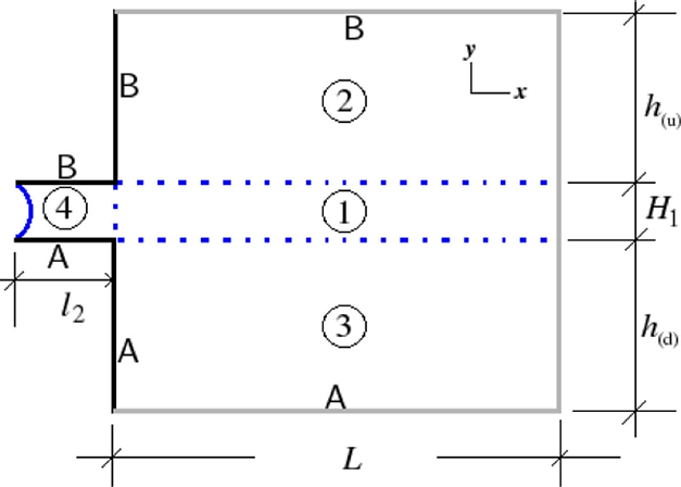
Figure 1 Diagram of a channel connected to an open domain. A pseudospectral method based on Chebyshev polynomials is used to calculate the numerical solution, which requires slicing the space into four rectangular subdomains. Dark lines correspond to solid walls, dotted lines are the intersections of the domains, and gray lines are open borders. A parabolic distribution of fluid velocity is imposed in the channel entrance (blue curved line).
For an incompressible fluid, the Navier-Stokes and continuity equations take the form
where Re = U H1/ν is the Reynolds number, ν is the kinematic viscosity and
An alternative way to study the flow in two dimensions is by using the vorticity-stream function formulation. To this end we introduce the stream function 12ψ, which is related to velocity by
Periodic driving is introduced by using the Dirichlet condition with a flow rate that varies sinusoidally in time according to
where t* is the dimensional time. To write this equation in dimensionless form we use the following relation between the representative velocity and the maximum flow rate: U = Q0/H1. From this definition, the dimensionless flow rate is
where S is the Strouhal number [Eq. (1)].
Equations (4) and (5) must satisfy the initial conditions and boundary conditions. For the initial conditions, the flow rate is set to zero so that both the stream function and vorticity vanish at t = 0. For the boundary conditions, we impose that the velocity vanish at solid boundaries. Because the stream function ψ is now the unknown, the no-slip condition must be given in terms of the flow rate Q(t). The condition that the normal component of velocity be zero at the boundary (un = 0) is equivalent to applying ψ = const., so we use ψ = 0 at the boundaries marked “A” (see Fig. 1) and ψ = Q at the boundaries marked “B.” In addition, a parabolic profile is imposed on the velocity field at the entrance of the channel (curved line at left of Fig. 1). The condition that the tangential velocity be zero (ut = 0) requires a more subtle treatment because it is equivalent to ∂ψ/∂n = 0.
Although solving Eq. (4) under the condition ψ = const. is sufficient, at this step we have no boundary condition for the vorticity equation. The usual procedure to overcome this difficulty is known as the influence matrix method11. In this method, a set of solutions for the vorticity equation-without the nonlinear term nor the terms evaluated at previous times-is calculated in a preprocessing stage. An individual solution is obtained by imposing ω = 1 at a point on the solid boundaries and ω = 0 elsewhere. Next, the solution of the full vorticity equation is calculated by imposing ω = 0 at all solid boundaries. The solution satisfying zero tangential velocity along the solid boundaries is obtained as a linear combination of the latter solution and the set of solutions obtained in the preprocessing stage. Finally, for the open boundaries, the Neumann condition is imposed (i.e., the normal derivatives of the stream function and vorticity are set to zero).
2.1. Methodology
The differential Equations (4) and (5) are solved by using the Chebyshev pseudospectral method for spatial coordinates, whereas a second-order Adams-Bashforth scheme is used to determine the temporal evolution11. The numerical methods and methodology used are the same as used by Lopez-Sanchez & Ruiz-Chavarria8. The mesh size is determined via the usual procedure: We begin with few points along the both x and y axis in all the domains shown in Fig. 1, and the number of points was increasing until no differences were obtained in the solutions in two successive refinements. Table I shows the number of spatial points used in the simulation for all domains shown in Fig. 1. We have verified that results are resolution independent from these refinements. To complete the description of the system the length and width of each domain are given in Table II.
Table I Number of points nx and ny for all domains shown in Fig. 1.
| Domain | nx | ny |
| ① | 300 | 80 |
| ② | 300 | 100 |
| ③ | 300 | 100 |
| ④ | 128 | 80 |
Table II Length of domains for different Strouhal numbers and for all domains shown in Fig. 1. In this case h = h(u) = h(d).
| S = 0:05 | S = 0:065 | S = 0:08 | S = 0:1 | |
| h=H1 | 9 | 9 | 9 | 9 |
| L=H1 | 28 | 28 | 25 | 20 |
| l2=H1 | 8 | 8 | 8 | 5 |
We use different Reynolds number for the numerical simulations; namely, 400, 700, and 1000. Because we are investigating interactions between dipoles, the choice of the Strouhal number becomes crucial. We use S = 0.05, 0.065, 0.08, and 0.10 to evaluate the effect of increasing Strouhal number. In all these cases, the dipole lifetime extends over several driving periods, allowing interactions between dipoles to arise in the different cycles.
3. Vorticity and dipole properties
In a periodic driving flow, a dipole is formed during each cycle. An issue raised in this work is the dipole lifetime. In most cases, the lifetime extends over several cycles, in which case two or more dipoles may coexist and interact. This interaction modifies dipole properties such as speed and vorticity and, in some cases, the vortices can coalesce. On the other hand Wells & van Heijst 14 have deduced that the condition S < 0.13 suffices for a dipole to escape. Their model is based on the assumption that all vorticity created inside the channel during the first half period (when flow rate is positive) is incorporated into the vortices. The aforementioned assumption is well satisfied for S ≳ 0.13. However, it is not valid for smaller values of S. In this case, a fraction of vorticity is not incorporated into the dipole, but forms instead a band in front of the channel output. A consequence is that dipole speed is lower than that predicted by the W-H model.
3.1. Interaction between vortices
For S < 0.13, the dipole created in the first driving period escapes the channel. But apart from this result and depending on the particular value of the Strouhal and Reynolds numbers, different scenarios may occur. For instance, under certain circumstances a vorticity band appears in front of the channel mouth and behind the dipole, in other cases the dipole is partially sucked back into the channel during the stage of negative flow rate, etc. The behavior of second and subs-equent dipoles depends not only on the dynamics of channel flushing into the open domain but also on the presence of dipoles created in previous cycles. Two conditions must be fulfilled to have dipole interaction: a) the dipole lifetime exceeds a driving period and b) the distance between two dipoles falls below a critical distance. In this section we present the most important results for interacting dipoles. Figure 2(a) presents the vorticity distribution corresponding to S < 0.08 and Re = 400 at t = 4.16T. Five dipoles are present. In addition, the distance between consecutive dipoles is not constant. Further evolution can be seen in Fig. 2(b), which corresponds to t = 6.56T. At this time, the first dipole is still present but the others, except the last one, have disappeared because of the combined action of viscosity dissipation and vortex interaction. The first dipole survives because the fluid in front of it is at rest and viscous dissipation is weak. The evolution of the second dipole (and subsequent dipoles) is as follows: it forms at the channel mouth, then detaches after a while, and finally moves away. As it moves, it is attenuated by viscosity until it finally disappears. In addition to the two vortices emerging from the channel, two vorticity spots appear as a result of the vorticity created into the channel during the return-flux stage of the previous period. This process is ilustrated in Fig. 3, where vorticity distribution inside the channel is plotted for three different times in the interval 1.90T < t < 2.35T. During the back flow some vorticity is created into the channel as shown in Fig. 3(a). A fraction of this vorticity is expelled out at the beginning of the next cycle (see Fig. 3(B) which finally forms the two spots (see Fig. 3(C)). These spots can be recognized by their opposite sign with respect to their partner vortex.
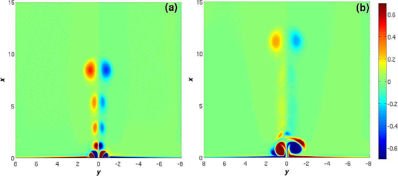
Figura 2 Vorticity distribution in X-Y plane for S = 0.08 and Re = 400. (a) A very symmetric vortex distribution appears at t = 4.16T. (b) t = 6.56T. Seven vortices have emerged, Only the first and the seventh are present. The first one survives because the interaction with other dipoles is weak and viscous dissipation is negligible. On the other the seventh dipole is in the stage formation.
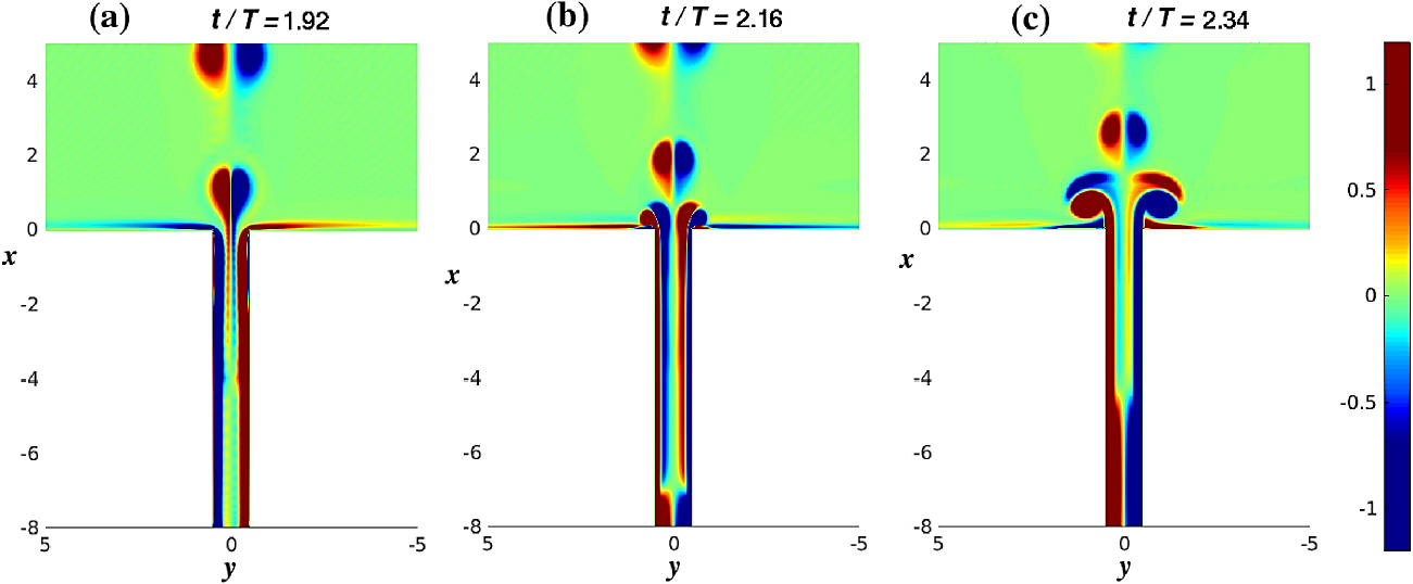
Figure 3 Vorticity distribution inside the channel for the interval 1.92T < t < 2.34T for S = 0.08 and Re = 400. a) During the stage of negative flow rate some vorticity is produced into the channel. This vorticity has a sign contrary to the vortex expelled at the beginning of the cycle, b) The vorticty created into the channel is expelled to the open domain, c) The aforementioned vorticity forms two spot in front of the vortices created during the present cycle.
To better understand the evolution of dipoles, Fig. 4 presents the position (x coordinate) of the second, third, and fourth dipoles for S = 0.08 and Re = 400. Each one moves with a decreasing velocity. The dipoles cannot move farther than a certain distance when they are blocked by the dipoles in front of them. At the end all these three dipoles are dissipated.
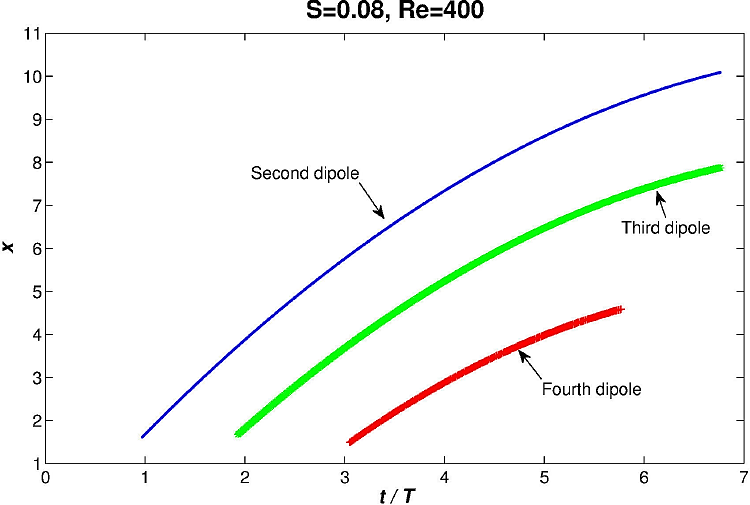
Figure 4 Position (x coordinate) vs time of second, third, and fourth dipoles for S = 0.08 and Re = 400. Except for the first, all dipoles stop because they are hindered by the previous dipole, which is in their path.
The solution differs for the same forcing (S = 0.08) but larger Reynolds number (Re = 700). Only every other dipole escapes with the remaining being sucked back in. Figure 5(a) shows the vorticity distribution for t = 1.8T; that is, during the negative flow rate of the second cycle. The first dipole is located at x ≈ 5 whereas the second dipole is being sucked back in. In addition two vorticity spots of opposite signs with respect the adjacent vortex are present. Figure 5(B) shows the vorticity distribution at t = 4.4T; that is, during the fifth cycle. As mentioned above, only the first, third, and fifth dipoles are apparent. The second and fourth dipoles have already been sucked back into the channel by the corresponding backflow. The first dipole moves away until the onset of the backflow, so it deforms but does not enter the channel. At the beginning of the next cycle, two vorticity spots appear in the vicinity of the channel output. These spots turn around the dipole, thereby reducing its speed, following which the second dipole moves slowly with respect to the first so that, after a half period, it is positioned where backflow effects are more intense. Thus, the second dipole moves toward the channel and is finally sucked in. The third dipole evolves similarly to the first one, and so forth. Finally, the fifth dipole has no well-defined form because it is still in the formation stage.
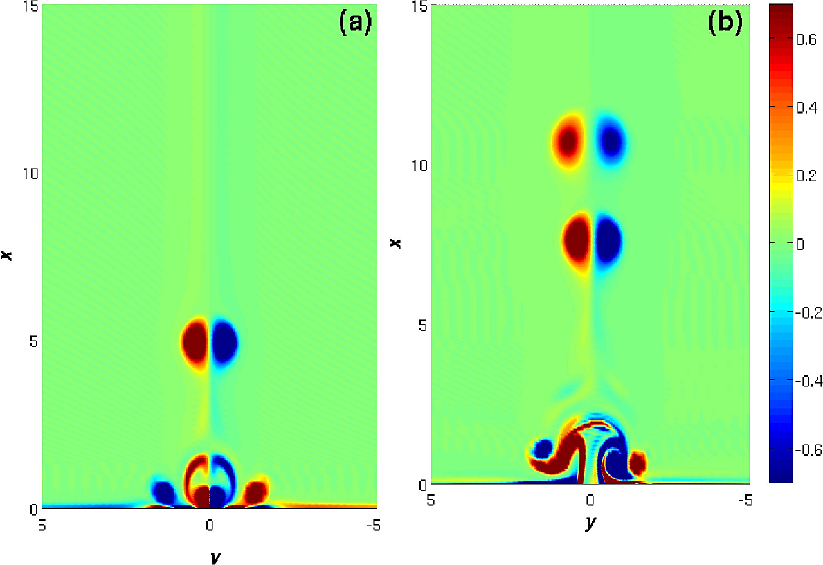
Figure 5 Vorticity distribution in X-Y plane for S = 0.08 and Re = 700. (a) At t = 1.8T, the second dipole is sucked back into the channel by the return flow. (b) t = 4:4T. The first, third, and fifth dipoles are shown. The second and fourth dipoles were sucked completely back into the channel by the return flow.
Increasing the Strouhal number S leads to a stronger interaction because the distance diminishes between successive dipoles. To support this statement, we present results for S close to the threshold of the W-H model. Figure 6(a) shows the vorticity distribution for S = 0.1, Re = 400 at t = 1.49T. Because this time corresponds to the second driving period, we see two dipoles. In addition, two vorticity spots appear in front of the dipole emerging from the channel. The same phenomenon also occurs in subsequent periods, as seen in Fig. 6(b). Although this figure corresponds to the seventh cycle (t = 6.7T), only two dipoles are apparent, the first and the seventh, the latter of which is being sucked back into the channel. In this case only the first dipole moves away from the channel, whereas subsequent dipoles are sucked back into the channel during the backflow, resulting in a concentration of vorticity near the channel output [see Fig. 6(b)]. This is a consequence of the interaction between consecutive dipoles. Multiple dipoles do not coexist in the proper sense because after the first one, the others fail to form.
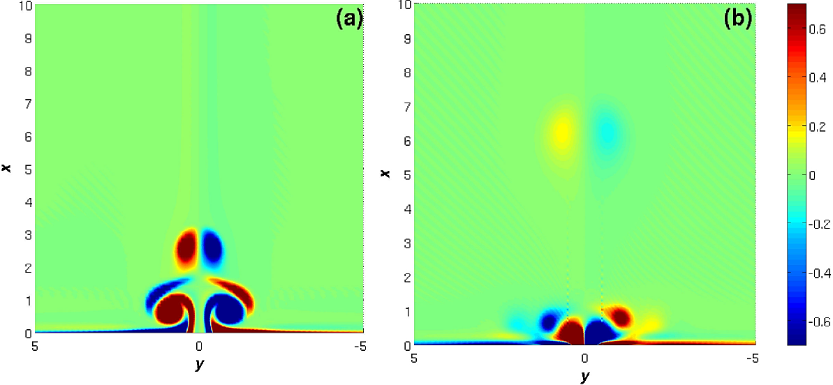
Figure 6 Vorticity distribution in X-Y plane for S = 0.1, Re = 400, and at (a) t = 1.49T and (b) t = 6.7T. Only the first dipole separates from the channel.
Another question raised in this paper is the symmetry of the flow. This symmetry depends both on the Reynolds and Strouhal numbers. Figure 7 shows a very symmetric distribution of vorticity for S = 0.065 and two different values of Reynolds number, namely Re = 700 and Re = 1000. The vorticity distribution corresponds to t = 3.47T. A different behavior happens for S = 0.08 and Re = 1000 as shown in Fig. 8. The figure shows the process of the lost of symmetry. Vorticity distribution corresponding to three different times are shown. In Fig. 8(a) and 8(b) (t = 1.4T and t = 3.6T respectively) the flow is symmetric. However, for t = 4, 2 (Fig. 8(c)) the symmetry is no longer conserved. The first dipole escapes the channel influence and remains aligned with respect to the symmetry axis. However, the symmetry of dipoles produced in the second and third cycles is broken, and the vortices do not follow the symmetry axis but take lateral trajectories until they are finally destroyed.
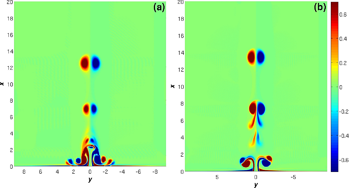
Figure 7 Vorticity distribution in X-Y plane for S = 0:065 at t = 3.47T and (a) Re = 700, (b) Re = 1000. To this point, symmetry is preserved in both cases.
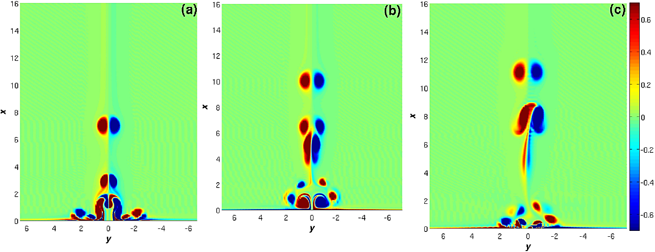
Figure 8 Vorticity distribution in X-Y plane for S = 0.08, Re = 1000. (a) t = 2.4T. The flow remains symmetric. (b) t = 3.6T. The flow begins to lose its symmetry and the second and third dipoles begin to coalesce. (c) t = 4.2T. All structures are nonsymmetric, even the first dipole. After a while, the second dipole reaches the first dipole, but the two do not merge.
Merger of dipoles
A possible scenario in a periodic driving flow is that dipoles created in two subsequent cycles approach each other, interact, and finally coalesce. Vortex coalescence occurs in this system in the form of a leap-frog process. Such a case is shown in Fig. 9 for S = 0.065 and Re = 400, which we consider to be the most representative. The vorticity distribution in Fig. 9(a) corresponds to the fourth period, so four dipoles are clearly recognized, but their intensities differ, which implies that they do not have the same speed. When the second dipole approaches the first, it enters a region where velocity field behaves like a jet. An enlarged view of the situation is shown in Figs. 9(b) and 9(c), emphasizing the coalescence phenomenon. Because the velocity is greater between the vortices of the dipole, an induced velocity acts on the second dipole, which modifies its shape so as to pass through the first dipole [Fig. 9(b)]. The induced velocity pulls the second dipole ahead of the first dipole [Fig. 9(c)] and then the two coalesce.
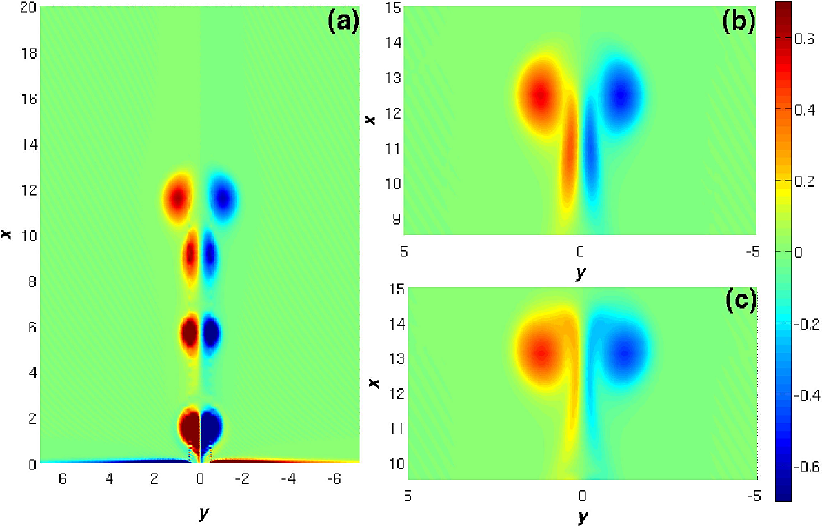
Figure 9 Vorticity distribution in X-Y plane for S = 0.065, Re = 400, and (a) t = 3.74T, (b) t = 4.23T, and (c) t = 4.6T. The first and the second dipoles coalesce.
Another case of vortex coalescence occurs for S = 0.08 and Re = 1000 during the fourth cycle (see Fig. 8, already presented in the previous section). As expected, because of a higher Strouhal number, coalescence occurs closer to the channel output than for the previous case. In Fig. 8(a), which corresponds to t = 2.4T, the first dipole is at approximately x = 7.5. The second dipole is close to the channel output (x ≈ 3) and the third dipole is in its initial stage. In Fig. 8(b), the symmetry starts to break down and the third dipole approaches the second dipole, deforms, and elongates. Coalescence begins but, at the end of the process, the flow is no longer symmetric, as depicted in Fig. 8(c). The merged dipole is not symmetric about the centerline and is approaching the first dipole.
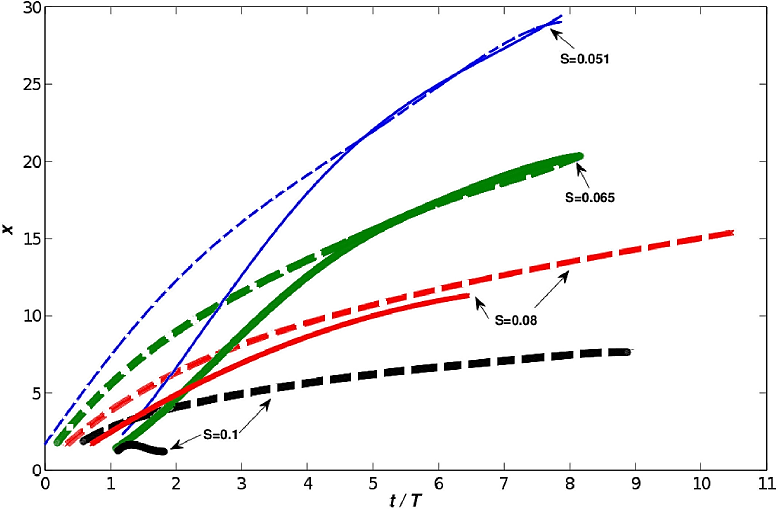
To better visualize the dipole coalescence in Fig. 10, we plot the position (x coordinate) of the first (dotted lines) and second (continuous lines) dipoles as a function of time for Re = 400 and all Strouhal numbers considered in this work. The first fact we notice is that the distance traveled by the dipoles decreases as the Strouhal number increases and, consequently, dipoles coalesce closer to the channel output as S increases. Conversely, the intersection of curves in Fig. 10 gives approximately the position and the time of coalescence (for a given Strouhal number). For S = 0.05, the second dipole catches up with the first at x = 20 and t = 5T, whereas for S = 0.065 the two dipoles coalesce at x = 13 and t = 4.5T. For S = 0.08, the continuous and dotted lines do not intersect, which means that the second dipole never catches up with the first. In this case the second dipole dissipates when it arrives at x ≈ 8, whereas the first dipole dissipates at x ≈ 15. When the Strouhal number reaches 0.1, only the first dipole detaches and subsequent dipoles are sucked into the channel, leading to a concentration of vorticity around the channel mouth 1.
3.2. Circulation
Based on the definition of circulation 3,4,5,7, we calculate this quantity in a domain containing a vortex (Γ) and also the circulation in the band formed in front of the channel (Γband). The goal is to evaluate how much vorticty created into the channel is incorporated to the dipole. With these results we can explain the discrepancies between the prediction of the W-H model and our numerical simulations for small values of the Strouhal number.
To calculate the circulation for the W-H model (ΓW-H), we use the suggestion 14
In our case, U(t) = U0 sin(2πt*/T). By integrating, we obtain
Then, the dimensionless circulation is
which is valid for t < 0.5T
The Fig. 11 shows the domains used to evaluate Γ and Γband for S = 051, Re = 1000 at t = 0.44T. The results are Γ = 1.156, Γband =0.6386, Γtotal =Γ + Γband = 1.7945; ΓW-H =2.4265. That means that in this case the numerical simulation underestimates the production of vorticity into the channel as compared with the W-H model.
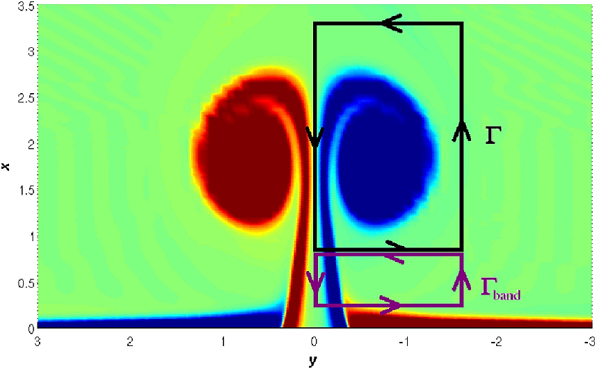
Figure 11 Circulation for the case S = 0.051, Re = 1000. The numeric total circulation Γtotal at time t = 0.44T is formed by the sum of the band (Γband) and the vortex (Γ) circulations. Γtotal is less than ΓW-H.
In order to have a knowledge of the vortex evolution the circulation was evaluated during the first half driving period for S = 0.05, S = 0.065, S = 0.08, and three different Reynolds numbers, namely Re = 400, Re = 700 and Re = 1000. Figure 12 shows these results and, for comparison, the prediction of the W-H model is included. Initially, all numerical curves have the same trend but, after t ≈ T/4 they begin to separate from each other. The biggest Reynolds number corresponds to the lowest circulation and vice versa. The discrepancy is due to the fact that in the case Re = 1000 the dipole moves faster than in the case Re = 400, therefore the vorticity has more time to incorporate in the latter case than in the first case. That is why the maximum value of the circulation is smaller for Re = 1000 than for Re = 400. Otherwise, for the three values of S considered in the figure, the numerical results for Γ and the prediction by the W-H model do not match; however, they have the same order of magnitude. For small t, the curve of the W-H model is proportional to t3 (as it will be shown in the next section) whereas the numerical data are proportional to t. The difference is related to how vorticity is created in the channel and expelled outward into the open area.
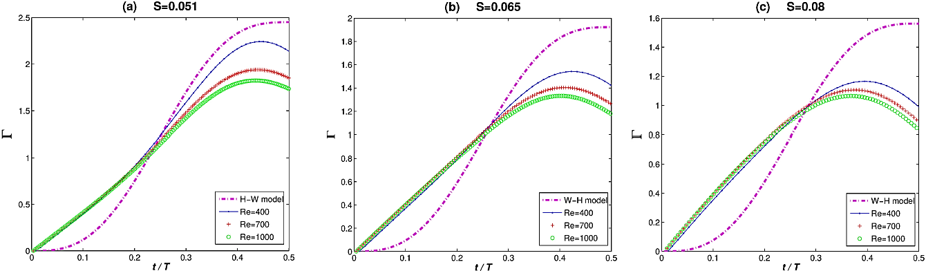
Figure 12 Circulation in half period for several cases and its comparison with the W-H model. Case Re=400, S = 0.051 shown in (a) is the most similar case to W-H model. While Reynolds number is smaller, the circulation is bigger
According to Lopez-Sanchez & Ruiz-Chavarria , for S = 0.05, the total vorticity obtained by numerical simulation exceeds that predicted by the W-H model, and Γband > Γ. That means that, for a Strouhal number less than 0.05, dipole speed is less than half that predicted by the model. In the present work, S ≥ 0.05, so discrepancies with the W-H model are smaller, although the vorticity band still appears.
Let us point out other features of circulation. First, Γ curves for a fixed Strouhal number are closer for S = 0.08 than for S = 0.05. This means that the circulation depends more weakly on the Reynolds number as the Strouhal number grows. Moreover, Fig. 12 shows that the maximum circulation happens before T/2 in the numerical simulations, whereas it occurs at T/2 in the W-H model. The viscosity is responsible for such behavior because the dissipation reduces the circulation.
Figure 13 plots the circulation of the first and second dipoles over a time interval lying in the second forcing cycle for S = 0.065 and Re = 400. In this interval, the first dipole is already formed and the second dipole is forming. For the first dipole, the maximum circulation is almost the same as that in Fig. 12(b). The circulation is less in the second dipole than in the first, which is explained by the presence of vorticity spots of opposite sign in the vicinity of the second dipole that are not present around the first dipole. The lower circulation in the second dipole is the reason why some dipoles for S < 0.13 are sucked during the stage of negative flow rate.
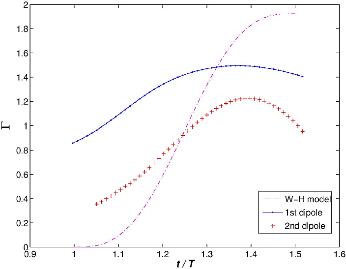
Figure 13 Circulation of one of two vortices in the first two dipoles vs t=T , for Re = 400, S = 0.065. The curve from the WH model is shown for comparison. The W-H model only works for the first driving period, so the W-H curve is intentionally shifted.
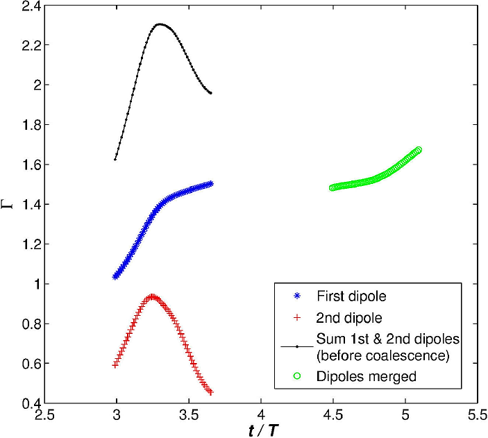
Another insight about the vortex coalescence comes from calculating the circulation before, during and after the coalescence in a symmetric and representative case: S = 0.065, Re = 400. Figure 14 shows the circulation of the first and second dipoles and their sum just before the dipoles coalesce, and after of this coalescence. The circulation of the merged dipole is lower than the sum of the first and second dipole circulation just before to coalesce. This fenomenon is due to the coalescence process leads to partial filamentation. These small scales filament leave the main structure, and they are eventually dissipated because of the viscosity. The result shows that the circulation is not conserved in the coalescence process for the viscous case.
4. Analytical Model
Wells & van Heijst 14 developed a model to describe the creation and evolution of dipoles in tidal-induced flow. In this model, the flow is composed of two point vortices and a time-dependent source. Their properties are those given by potential theory, so no dependence on Reynolds number appears because the viscosity is not taken into account. First, in this model the dipole moves with a speed of
where Γ is the circulation of a single vortex and d is the distance between vortices. The vorticity that feeds the dipole is created inside the channel. To evaluate the circulation we use dimensional arguments: First, the vorticity in the channel is of the order of ω ≈ U/(2δ), δ is the thickness of the boundary layer. Then, if we assume that all vorticity created in the channel is incorporated into the dipole, the circulation Γ is the surface integral of ω over the area covering all fluid leaving the channel. Because U is time dependent, Γ is calculated by
During positive flow rate, Γ grows because the vorticity leaving the channel is continuously incorporated. If we normalize t by the period T and let the velocity in the channel output be U(t) = sin(2πt)/S, then the position x(t) and velocity ud(t) of the dipole during the stage of positive flow rate (t < 1/2) are
Both equations are valid provided that all the vorticity created in the channel is incorporated into the dipole. The results obtained in a previuos work 8 indicate that Eqs. (10) and (11) are asymptotically recovered when S → 0.13, but this does not happen when S → 0. The discrepancy for small S arises from the fact that the dipole speed (ud(t)) given by Eq. (11) exceeds, at a certain time, the fluid velocity U(t) at the channel mouth. If ud(t) > U(t), then the vorticity created in the channel is no longer incorporated into the dipole. This can be seen in Fig. 15, which shows both the velocity of the fluid at the channel mouth (U) and the dipole speed ud (both multiplied by S) as a function of time for S=0.0075 and S = 0.1. For S = 0.0075, both curves intersect at tc = 0.14, and for S = 0.1 the intersection happens at tc = 0.43. Roughly, this value of t gives the upper limit of the interval during which vorticity leaving the channel is incorporated into a dipole. Consider the case S = 0.0075. Initially, flow velocity exceeds dipole speed, so fluid particles leaving the channel reach the dipole and consequently vorticity is incorporated into the dipole. However, according to the W-H model, the dipole speed increases continually until the end of the half period, leading to the prediction ud ≫U. This is not true because, when ud > U, the particles transporting vorticity cannot reach the dipole. If the circulation no longer increases, the dipole speed attains a constant value, which is roughly that of the intersection of curves in Fig. 15 (i.e., when U = ud ):
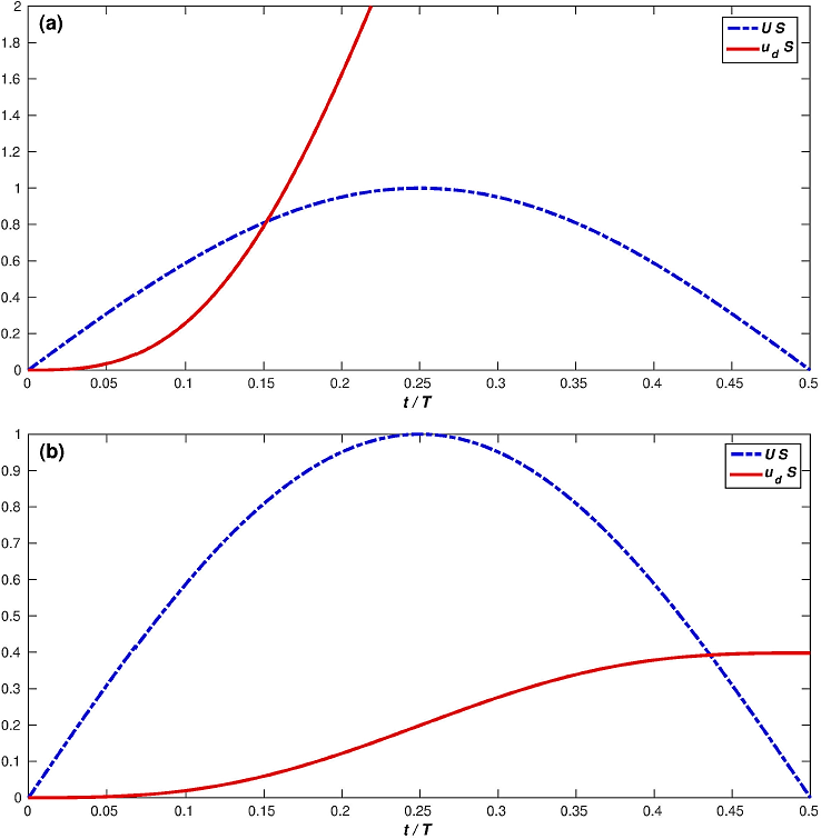
Figure 15 Flow velocity at channel output (dashed line) and dipole speed (solid line) vs time for (a) S = 0.0075 and (b) S = 0.1. Both quantities were multiplied by S to have a maximum flow velocity equal to 1.
To estimate this speed we must determine the root of Eq. (12). To this end we Taylor expand both sides of this equation to third order, which gives
Substituting this time into Eq. (11) gives the speed of the dipole. To calculate the position of the vortex at t = tc we use Eq. (10). Another possibility is to Taylor expand this equation, which gives a first nonvanishing term of the order four and then the dipole position is
Consequently, the position k at which dipole attains a constant speed is
Equations (13)-(15) are valid provided S → 0. In this case, time tc is small, so the Taylor expansion to third or fourth order provides a good estimate of the original functions. Table III gives the values of tc for various S. If we calculate the root of Eq. (12) instead of using a Taylor expansion, we find that Eqs. (13)-(15) provide a good estimate when tc = 0.25. In this respect, the value for tc predicted with S = 0.1 by Eq. (13) is tc = 0.32 (see Table III), which differs from the value of 0.43 calculated directly from Eq. (12).
Table III Comparison of different distances over which dipoles move in T/2 as given by W-H model (DW-H), our correction (D), and the numerical simulations (Dnum). The time tc after which vorticity is no longer incorporated into the dipole and the constant velocity u(tc) reached by the dipole are also included.
| S | tc | u(tc) | DW-H | D | Dnum |
| 0.0075 | 0.14 | 87.5 | 176.8 | 35.1 | 23.6 |
| 0.01 | 0.158 | 68.1 | 99.5 | 26.6 | 19.36 |
| 0.025 | 0.224 | 25.3 | 15.9 | 9.1 | 5.802 |
| 0.051 | 0.28 | 8.9 | 3.8 | 3.2 | 1.91 |
| 0.065 | 0.29 | 6.3 | 2.4 | 2.2 | 1.42 |
| 0.08 | 0.31 | 9.5 | 1.55 | 1.56 | 0.96 |
| 0.1 | 0.32 | 3.0 | 1.0 | 1.1 | 0.78 |
| 0.11 | 0.32 | 2.54 | 0.82 | 0.92 | 0.67 |
| 0.15 | 0.34 | 1.44 | 0.44 | 0.53 | 0.48 |
The value of k depends on S but, in any case, k ≤ (3/2)π = 4.71. Dipoles evolve over three stages. In the first stage, the circulation of vortices, Γ, is well described by the W-H model, and the dipole position is proportional to t4. In the second stage, the velocity is sufficient to prevent a further dose of vorticity from arriving from the channel. The dipole speed is essentially constant. In the final stage, after t > (T/2), the dipole is affected by the negative flow rate.
The W-H model is recovered asymptotically when S → 0.13, which can be justified with the help of Fig. 15(b). This figure shows that two curves intersect when the dipole speed is near its maximal value. For t > tc no additional vorticity is incorporated into the dipole, although this fact has small effect on the dipole speed.
After a half cycle has elapsed, the dipole position is
Table III compares data corresponding to this model with the results of the W-H model and of our numerical simulation. Also included in the table is the time tc, the velocity u(tc) of the dipole, and the distance traveled after a half period according to our model (D), the W-H model (DW-H), and the numerical simulations (Dnum).
These results show that the dipole position after a half period is overestimated by a factor five by the W-H model for S = 0.0075. For higher values of S, this overestimate becomes less important. The modification of the W-H model does not modify the criterion given by these authors regarding the condition for a dipole to escape because, for S = 0.13, the dipole does not reach the position x = k.
5. Some comparative data
We compare dipole displacement obtained numerically in this work with data obtained by observation 1 and experiment 9. To begin, we estimate the distances between dipoles and the channel in Fig. 7 of Ref. 1, which is for S = 0.05; the results are d1 ≈ 6.9 and d2 ≈ 2.8. Our numerical simulation gives d1 = 7.68 and d2 = 2.3, for Re=400. Note that two important differences exist between these two results: First, according to the satellite pictures in Ref. 1 the channel length is small as compared with the channel width H1. Second, the dipoles in Ref. 1 lose their symmetry and are displaced less than in our numerical simulation because other currents are involved in the system. Thus, the main comparison is qualitative, in the sense of the coexistence of multiple dipoles.
We made also a comparison with two cases of Nicolau del Roure 9; namely, S = 0.11 and S = 0.06. At t = 0.35T, the distance between dipole and channel output is d1 = 1.07 in the Nicolau experiment (Fig. 5 of Nicolau del Roure et al., 9, corresponding to S = 0.11), and d1 = 1.61 in our numerical simulation. At the same time but for S=0.06 (Fig. 8 of Nicolau del Roure et al., 9), the dipole position is d1 = 1.58, whereas the numerical simulation gives d1 = 1.43. In both numerical cases Re = 400.
6. Conclusions
This paper presents the results of some numerical simulations of a periodic flow between a channel and an open domain. The ultimate aim is to understand the formation mechanisms of multiple dipoles and the interactions between such dipoles. Each cycle produces a dipole; if the dipole lifetime exceeds a period, two or more dipoles may coexist, which opens the door for interactions between vortices. In some cases this interaction leads to dipole coalescence. Such phenomenon occurs as a leap-frog process when dipoles approach each other. In addition to the vortex merger, another phenomenon is observed, that is, the formation of the vorticity spots in front of the dipoles leaving the channel. In some circumstances these spots are responsible for the fact that half of the dipoles are sucked back into the channel and the remaining dipoles escape. This behaviour occurs because when a dipole forms, the spots (which are in fact small vortices) move around it, thereby reducing its translational speed. Next, at the end of a half period, the vorticity spots are sucked back into the channel. The next cycle produces no vorticity spots, so the dipole can escape.
A result that has been highlighted in the paper is that for a flow with a Strouhal number below the critical value 0.13 not all vorticity created in the channel is incorporated into dipoles. The fraction of this vorticity grows as S → 0. A consequence is that the W-H model overestimates the speed attained by the dipole. Based on this results we have proposed an analytical model that provides results that are more consistent with experimental and numerical data than those of the W-H model. On the other hand, we could expect that the numerical results approach the W-H model when the Reynolds number grows, because that model is inviscid. This happens only during the first stage of the dipole evolution. After there is a discrepancy because the emergence of the vorticity band behind the dipole. The aforementioned discrepancy diminishes when S → 0.13.
Another important conclusion is that the evolution of the first dipole is consistent with the W-H model in the sense that, when S < 0.13, the dipole moves away from the channel. However, the results for S = 0.1 show that subsequent dipoles are sucked back into the channel during backflow and that, as a consequence, vorticity is concentrated near the mouth of the channel.
Finally, when the Reynolds number increases, symmetry is broken and vortices destroy by a combined a action of viscous dissipation and the growth of instabilities. Although the Reynolds number used in these simulations differs from what is found in coastal systems and these simulations do not consider the Coriolis force, the results are consistent with observations reported in the literature, such as the coexistence of multiple dipoles 1.

