1. Introduction

Nonlinear partial differential equations (NPDE) have been analyzed by different type of mathematical approach, among which include the Darboux transformation, the inverse scattering method, the Hirota method, the Backlund transformation, the tanh method, the sine-cosine method, the exp-function method, the variational iteration method, the homogenous balance method and among others ^1-41.

In this article, the D(m, n) system ¹ are considered:

For m = 2 and n = 1, the system (1) is called “The normal Drinfel’d-Sokolov system”

where a, b, c are unchanged. The system (2) is considered as an example of a system of nonlinear equations possessing Lax pairs of a special form ¹³. Wang obtained its Hamiltonian, recursion, symplectric and cosymplectric operators and roots of its symmetries and scaling symmetry of the system (2) ¹⁴.

For n = 1 the system (1) changes to “The generalized Drinfel’d-Sokolov system” as:

Wazwaz obtained some exact traveling wave solutions of the D(m, n) system with compact and noncompact structures by applying the tanh method and the sine-cosine method ¹⁵.

We firstly apply the ansatz method ^{16,17,18,19,20} to obtain the exact special solutions to the D(m, n) system. Then, we use the He’s variational approach ²¹ to obtain unknown traveling wave solution to the subsidiaries of the D(m, n) system. We give a comparison between the obtained solutions and those exist in the literature.

2. Ansatz method

We start by considering the solution of the equation

where a₀ ≠ 0 and b₀ ≠ 0 are constants. When b₀ > 0, Eq. (4) admits two solutions as:

where A is an arbitrary unchanged. If b₀ < 0, recognizing that cosh² z + sinh² z = 1 we know that Eq. (4) has two solutions of the form as:

Secondly, we make a consideration of the solutions of the equation of the form

where c₀ ≠ 0 and d₀ ≠ 0 are constants. If c₀ < 0, Eq. (7) confesses two solutions

If c₀ > 0 in Eq. (7), then the equation offers two solutions of the form

2.1. Nonlinear Dispersion D(m, n) System

We assume that the traveling wave solution has the form u(x, t) = u(ξ) with wave variable ξ = k(x - λt), (k, λ ≠ 0). Then, we get the following ordinary differential equation:

-kλu'+kνm'=0, (10)

-kλν'+ak3νn‴+bku'ν+ckuν'=0. (11)

We get

u=1λνm+c1, (12)

by (11), where c₁ is arbitrary constant. Substituting (12) into (11) we obtain

(13)

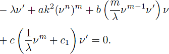
By integrating Eq. (13), we get

(cc1-λ)ν+ak2(νn)″+bm+cλ(m+1)νm+1=c2. (14)

where c₂ is integration constant.

Case 1. When c = -bm = λ/c₁, the nonlinear ODE (14) becomes

ak2(νn)″-c2=0. (15)

Therefore, we get the rational solution of Eq. (15),

ν(x,t)={c22ak2(x-λt)2+c3(x-λt)+c4}1n, (16)

and

u(x,t)=1λ{c22ak2(x-λt)2+c3(x-λt)+c4}mn+c1, (17)

where c₃ and c₄ are arbitrary constants.

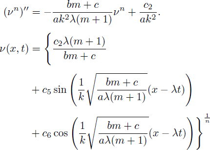
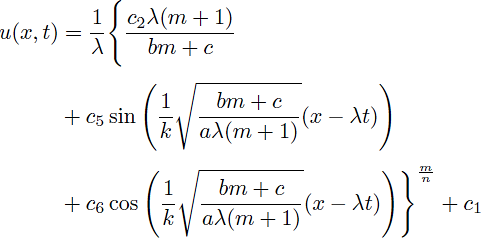
Case 2. If we take m = n - 1 and c = λ/c₁ in Eq. (14), the following traveling wave solutions are obtained

(18)

and

(19)

where c₅ and c₆ arbitrary constants. In view of (18) and (19), we clearly see that these solutions exist provided that (bm + c)/(aλ(m + 1)) > 0

(20)

and

(21)

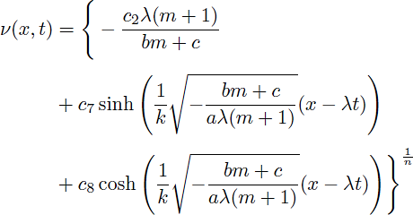
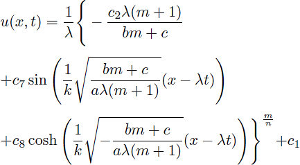
where c₇ and c₈ arbitrary constants. In view of (20) and (21), we clearly see that these solutions exist provided that (bm + c)/(aλ(m + 1)) < 0.

Case 3. c + bm ≠ 0, cc₁ - λ ≠ 0 and specially c₂ = 0.

Let

dνndξ=z, d2νndξ2=zdzdνn. (22)

Substituting (22) into (14) leads to the following equation

(23)

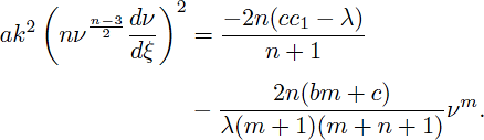
Letting ν = w^2/m, we have

ν=w2m⇒dv=2mw2m-1dw, (24)

which changes Eq. (23) to

(25)

If we take n = 2m + 1 in Eq. (25), we get the algebraic traveling wave solution of the form:

ν(ξ)=1B(A-B2ξ2-2B2ξC-B2C2)1m, (26)

and

u(ξ)=1λB(A-B2ξ2-2B2ξC-B2C2)+c1, (27)

where

A=-(cc1-λ)m24ak2(m+1)(2m+1)

and

B=m2(bm+c)2ak2λ(m+1)(3m+2)(2m+1).

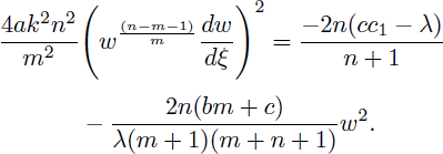
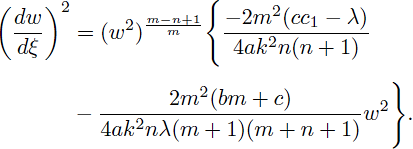
Case 4. If m = n - 1, we know that Eq. (25) becomes

(28)

where n ≠ 1 and a, k, n, λ ≠ 0.

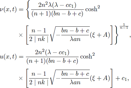
If we take anλ(c + bn - b) > 0, then we acquire from Eqs. (5) and (28)

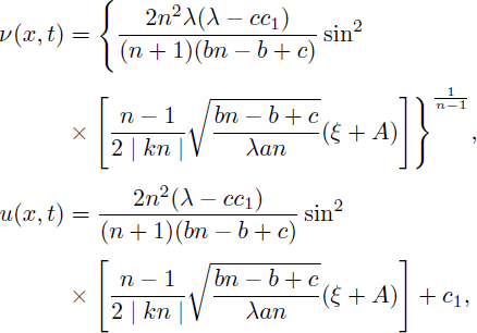(29)

and

(30)

Theorem 1. The D(m, n) system has solutions in Eq. (28) described as follows:

1. When anλ(c + bn - b) > 0,

ν=*20c2n2λ(λ-cc1)(n+1)(bn-n+c)cos2n-12∣kn∣bn-b+cλan(ξ+A)1n-1,∣b0(ξ)∣≤π2,0,Otherwise (31)

is a solitary wave solution with compact support.

2. When anλ(c + bn - b) > 0,

ν=*20c2n2λ(λ-cc1)(n+1)(bn-n+c)cos2n-12∣kn∣bn-b+cλanξ+A1n-1,0≤∣b0(ξ)∣≤π,0,Otherwise (32)

is a compacton solution for Eq. (1) and

b0=n-12∣kn∣bn-b+cλan.

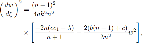
3. Equation (25) can be written as following

(33)

If n = 1in Eq. (33) that yields as

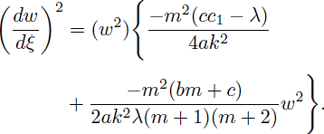(34)

When a(cc₁ - λ) < 0,

(35)

which is a singular soliton solution for the D(m, n) equation for

0<ξ<πm2k(cc1-λ)a

4. When a(cc₁ - λ) > 0 and m < 0,

(36)

is a traveling wave solution for the D(m, n) equation for

ξ<πm4k(cc1-λ)a.

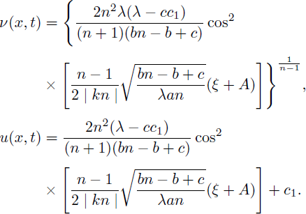
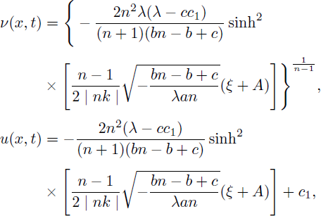
Remark 1. If (bn - b - c)/(λan) < 0, it follows from (6) and (28) that

(37)

and

(38)

Theorem 2. The D(m, n) equation with when m = n equation has the following solutions:

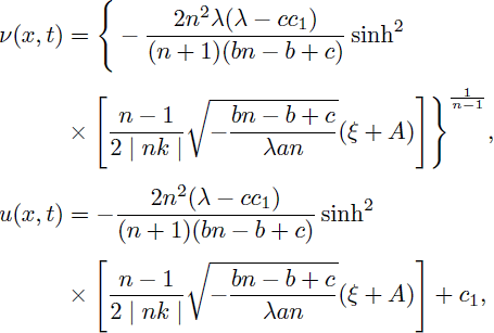
1. When (c + bn - b) < 0, anλ > 0, (λ - cc₁)(n + 1) < 0 and n ≠ 1

(39)

is a solitary solution of Eq. (1).

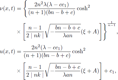
2. When (c + bn - b) < 0, anλ > 0, (λ - cc₁)(n + 1) > 0 and n ≠ 1

(40)

is a solitary solution of Eq. (1). If we take n < 1, then Eq. (40) is a bounded solution.

3. m = n < 1solutions (39) and (40) turns to solitary wave solutions

(41)

and

(42)

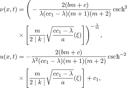
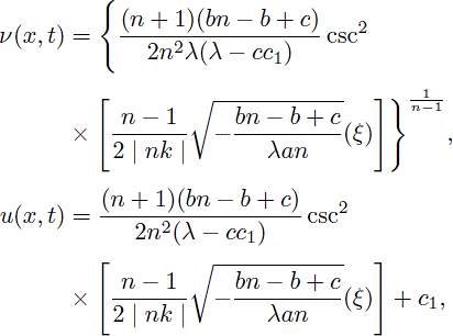
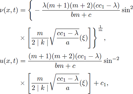
Case 5. a(cc₁ - λ) > 0 and m > 0,

Thus, by using (8) and (34), the periodic solutions of Eq. (1) are obtained as:

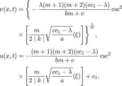(43)

and

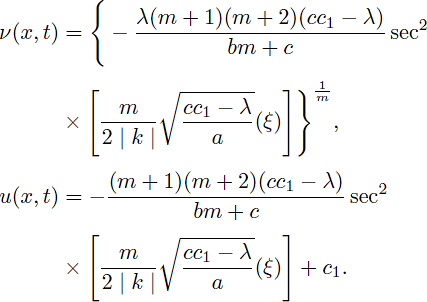(44)

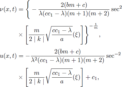
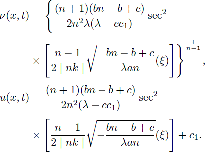
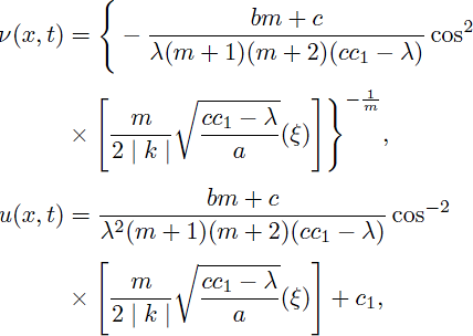
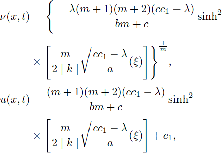
Case 6. a(cc₁ - λ) > 0 and m > 0,

Therefore, by considering (9) and (34), solitary pattern and bell-shaped solitary wave solutions of (1) are obtained as:

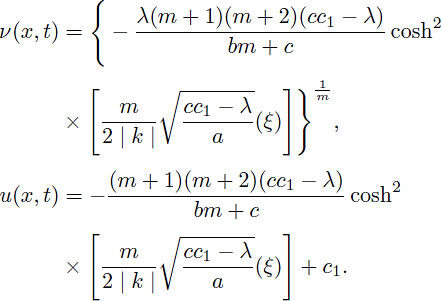(45)

and

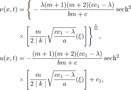(46)

Case 7. a(cc₁ - λ) > 0 and m ≠ 0,

Using the solutions of (43) and (44), gives the following compacton solutions as:

(47)

for

0≤πm2k(cc1-λ)a|≤π2

and u = 0, otherwise.

(48)

for

0≤|πm2k(cc1-λ)a|≤π

and u = 0, otherwise.

Case 8. a(cc₁ - λ) > 0; m < 0 and m ≠ 1.

Using cosh(x) = cos(ix) and sinh(x) = -sin(ix) we have the following solitary pattern solutions of Eq. (1):

(49)

and

(50)

Remark 2. When m = n < 1, the obtained solution (42) agrees with the outcomes (2.13a), (2.13b) in ³⁶ and (25) in ³⁷. The solution (42) changes to the compacton solution (2.12a) and the periodic solution (2.12b) in ^36,37.

If m > 0, the obtained solution (46) is consented with the outcomes (3.18a) and (3.18b) described in ³⁶ and (26) in ³⁷. The solution (46) changes to the solitary pattern solution (3.17a) and solitary wave solution (3.17b) in ³⁶.

Remark 3. If a(cc₁ - λ) < 0, the obtained solution (35) agrees with the outcomes (3.9a) and (3.9b) in ³⁶ and (32) in ³⁷. The solution (35) changes to the singular solitary wave solution.

Remark 4. If we take (c + bn - b) < 0, anλ > 0, (λ - cc₁)(n + 1) < 0 then the obtained solution (39) similar to the solitary pattern solutions (3.7a) and (3.7b) in ³⁶ and (46) in ³⁷.

3. Variational principle

In this Section, He’s variational principle will be applied to the system (1). This technique was first proposed by He²¹ and it is popularly known as He’s semi-inverse variational principle. Some years back, it was applied mainly to extract soliton solutions of nonlinear PDEs and systems by many authors ^{16,17,18,19,20,21,22,23,24}. Biswas and co-workers ^17,18,19,20 obtained optical solitons and soliton solutions with higher order dispersion by applying the He’s variational principle. Xu and Zhang’s²⁵ used a variational principle to construct catalytic reactions in short monoliths by He’s semi-inverse approach. He’s variational method was used to the effective nonlinear oscillators with high nonlinearity by Liu ²⁶. Zheng et al. ²⁷ established a class of generalized variational principles for the initial-boundary value problem of micromorphic magneto electrodynamics by He’s semi-inverse technique. In order to seek traveling wave solutions of the system (1). We consider

Let νⁿ = V

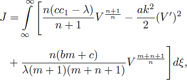(52)

the 1-soliton solution ansatz, given by

is substituted into (51). Here, in (53), the parameters p and q represent the amplitude and inverse width of the soliton, respectively.

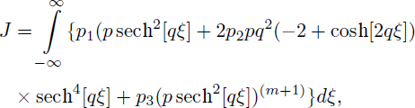(54)

where p₁ = cc₁ - λ, p₂ = ak² and

From the above equation it is obtained as

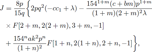(55)

where F is Gauss’ hypergeometric function defined as

and Re[(2 + m)q] > 0, Re[(1 + n)q] > 0, Re[q] > 0.

Making J stationary with respect to p and q results in

(57)

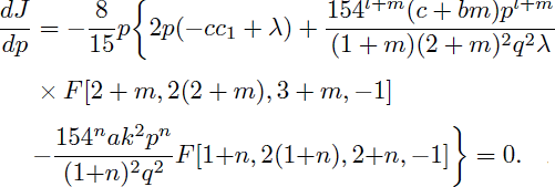(58)

Solving Eqs. (57) and (58) for m = n = 2 simultaneously, we get

Therefore, by substituting p and q in (52) we have the following a new solitary wave solution for the system (1) as:

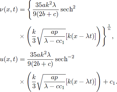(60)

So, the solitary wave solution (60) will exist for ap(λ - cc₁) > 0.

4. Results and Discussions

In this article, we investigated the nonlinear dispersion D(m, n) system and obtained some traveling wave solutions by applying the ansatz technique and the He’s variational principle. Several forms of solutions including topological, non-topological, compacton, solitary pattern, singular soliton, algebraic and periodic wave solutions were acquired. The approaches can be used to a lot of other nonlinear differential equations and coupled systems. Some new obtained exact solutions were previously unknown by other methods. We proved the existence of these solutions for a generalized form of the D(m, n) system under specific conditions. In general, the outcome expose that the ansatz approach and the He’s variational principle are important mathematical techniques for solving nonlinear partial differential equations in terms of correctness and ability to avoid errors.