


 nueva página del texto (beta)
 Inglés (pdf)
 Artículo en XML
 Referencias del artículo
 Enviar artículo por email
 Citado por SciELO
  Similares en
SciELO
Similares en
SciELO 
 Permalink
1. Introduction
Finding exact solutions of nonlinear differential equations has long been an active field of research because of the insight they offer in the understanding of many processes in physics, biology, chemistry, and other scientific areas. Among the methods developed to find analytical solutions of nonlinear ordinary differential equations (ODEs) and nonlinear partial differential equations (PDEs) we enumerate the truncation procedure in Painlevé analysis1, the Hirota bilinear method2, the tanh function method3,4 , the Jacobi elliptic function method5, and the Prelle-Singer method6,7.
The factorization method, which in mathematics has roots that go to Euler and Cauchy, is a well-known technique used to find exact solutions of linear second order ODEs in an algebraic manner. In physics, it has attracted much interest as an elegant way of solving fundamental eigenvalue problems in quantum mechanics8-14, and later due primarily to its natural association with supersymmetric quantum mechanics. The latter approach has been extended to some types of nonlinear ODEs15, and to more dimensions16-19 as well. In recent times, the factorization technique has been applied to find exact solutions of many nonlinear ODEs20, and to nonlinear PDEs, mainly in the context of traveling waves21-29. The factorization technique was further extended to a class of coupled Liénard equations, which also included a coupled version of the modified Emden equation, by Hazra et al30. Their algorithm can be generalized to higher order scalar and coupled ODEs, but one has to pay the price of increased algebraic complexity. In addition, Tiwari et al31 factorized even more complicated quadratic and mixed Liénard-type nonlinear systems, among which the coupled Mathews-Lakshmanan nonlinear oscillators.
In this paper, we generalize the factorization technique that we introduced previously22,23 for nonlinear equations with a monomial function in the first derivative, i.e., with a damping term which can be also nonlinear, to nonlinear equations with polynomial functions of second and third degree in the first derivative. In the following section, we review the factorization in the monomial case. Next, we present the factorization of nonlinear equations with polynomial function of second degree in the first derivative and illustrate it with a couple of examples. The last section is devoted to the factorization of nonlinear equations with polynomial function of third degree in the first derivative. We end up the paper with the conclusion section.
2. Factorization of nonlinear equations with a monomial of first degree in the first derivative
Nonlinear equations of the type
where the subscript s denotes the derivative with respect to 𝑠 and 𝐹(𝑦,𝑠) and 𝑓(𝑦,𝑠) are arbitrary functions of 𝑦(𝑠) and 𝑠, can be factorized as follows32:
where 𝐷 𝑠 =𝑑/𝑑𝑠. Expanding ([n2]), one can use the following grouping of terms22,23:
and comparing Eq. (1) with Eq.(3), we get the conditions
Any factorization like (2) of a scalar equation of the form given in Eq. (1) allows us to find a compatible first order nonlinear differential equation,
whose solution provides a particular solution of (1). In other words, if we are able to find a couple of functions 𝜙 1 (𝑦,𝑠) and 𝜙 2 (𝑦,𝑠) such that they factorize Eq. (1) in the form (2), solving Eq. (7) allows to get particular solutions of (1). The advantage of this factorization has been shown in the important particular case when there is no explicit dependence on 𝑠, i.e., for equations
for which the factorization conditions are
when the two unknown functions 𝜙 1 (𝑦) and 𝜙 2 (𝑦) can be found easily by factoring 𝐹(𝑦) when it is a polynomial or written as a product of two functions. This property of the nonlinear factorization has been successfully used when it has been introduced a decade ago and contributed to its popularity33. An illustration of this technique in the case of the cubic Ginzburg-Landau equation can be found in34. Notice that interchanging the factoring functions turns (8) and (9) into
which correspond to equations
If 𝑠 is a traveling variable, this suggests kinematic relationships between the kink solutions of (7) and (12) evolving under the different nonlinear dampings 𝑓(𝑦) and 𝑓 (𝑦).
Finally, in the case 𝑓=0 and 𝐹(𝑦,𝑠)=𝑉(𝑠)𝑦, the factoring functions 𝜙’s depend only on 𝑠 and the equations ([n1]) are linear ones
The factorization conditions take the simplified form
From (14), one has 𝜙 1 =− 𝜙 2 =𝜙 which upon substitution in (15) leads to the well known Riccati equation −𝑑𝜙/𝑑𝑠− 𝜙 2 =𝑉(𝑠) defining the Schrödinger potential in quantum mechanics in terms of the factoring function. The interchange of 𝜙 1 with 𝜙 2 produces the partner Riccati equation 𝑑𝜙/𝑑𝑠− 𝜙 2 = 𝑉 (𝑠) of much use in supersymmetric quantum mechanics35,36.
3. Factorization of nonlinear equations with polynomial function of second degree in the first derivative
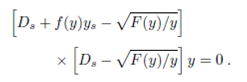
Let us consider the following nonlinear second order ODE with variable coefficients
A factorization of the form
is possible if the following constraint equations are satisfied:
There are also cases when one can work with 𝜙 2 =0. In such cases, the constraint equations take the form
Finally, the degenerate case corresponding to 𝜙 1 =0, which also implies 𝐹=0, leads to the simple constraint
As an example of a degenerate case, we mention the equation for the radial function of the isotropic metric in general relativity37
for which (22) is written as
The solution
where 𝑎 and 𝑏 are integration constants, can be found by elementary means37.
The most important application is when no explicit dependence on 𝑠 occurs in the equation and so neither 𝐹 nor the 𝜙’s depend on 𝑠 when the constraints are similar to (8) and (9). If moreover one assumes 𝜙 1 = 𝜙 2 =𝜙 then the second constraint equation provides the factorization function as
Substituting (26) in the first constraint equation leads to the following expression for the 𝑔 coefficient
For given 𝑓(𝑦) and 𝐹(𝑦), the latter equation gives the coefficient 𝑔(𝑦) for which the nonlinear equation can be factorized in the form
 (28)
(28)
There are equations of the latter type which do not present a linear term in the first derivative. This implies 𝑔(𝑦)=0, i.e.
which is separable. The solution
with 𝐶 an integration constant, provides the form of 𝐹 which for given 𝑓 allows the factorization of the equation. However, as simple as it may look, the condition ([C6]) is quite restrictive.
In physical applications, differential equations with squares of the first derivative are encountered in highly nonlinear areas, such as cosmology and gravitation theories, e.g., Weyl conformal gravity and 𝑓(𝑅) gravity , but occasionally they show up in other branches as well. In the following, we will give two examples of factorization of such equations.
3.1 An equation in Weyl’s conformal cosmology
The following equation
where 𝛼 and 𝜎 are real constants, arises in intermediate calculations concerning the vacuum solution of the field equations in Weyl’s conformal gravity . Let us try the factorization
Therefore, the following constraint equations should be satisfied
 (33) , (34)
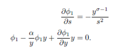
Equation (34) is separable and generates the function 𝜙 1 (𝑦,𝑠)=𝑓(𝑠) 𝑦 𝛼−1 , then, from Eq. (33) we obtain
which implies 𝛼=𝜎, and 𝑓(𝑠)= 1 𝑠 + 𝑐 1 , where 𝑐 1 is an arbitrary constant.
Assuming the following27
then, we get
with solution 𝛺= 𝑘 0 𝑦 𝛼 . Therefore, we get the first order equation
which can be rewritten in the form
where 𝑘 1 is an integration constant. The general solution of Eq. ([Peq11b]) is given in the form
where 𝑘 2 is an integration constant. For 𝑘 1 =0 and 𝛼=5, we obtain the following particular solutions
 (41) , (42)
3.2 Langmuir-type equations
A particular example of the type (16) is the following equation
which when 𝛾=4/3 provides Langmuir’s radial 𝛽 function occurring in the formula for the space charge between coaxial cylinders . Using ([eq4c]), one can choose
Substituting (43) in (18), one obtains 𝛾=5/3, which shows that the Langmuir case cannot be factored. If 𝛾=5/3, we can obtain a particular solution from the first-order differential equation
which is
where 𝐶 is the integration constant.
4. Factorization of nonlinear equations with polynomial function of third degree in the first derivative
It is well known that equations of the type
where the coefficient functions are mappings from two-dimensional disks to the set of real numbers, 𝒟 2 →ℝ, define projective connections .
Such equations allow for the factorization
with the compatible first order equation
under the constraint equations
On the other hand, for any symmetric affine connection 𝛤=( 𝛤 𝑗𝑘 𝑖 (𝑠,𝑦)), the so-called projective connection associated to 𝛤 which carries all information about unparametrized geodesics of 𝛤 is determined by the equation
Thus, one finds that equations (52) can be factored if
We do not present any particular case. Rather we notice that for given 𝛤’s, (53) provides 𝜙 1 . Then, substituting in (54), we get 𝜙 2 , but in the end (55) should be still satisfied. This looks complicated and makes the success of the method less probable.
5. Conclusion
In summary, we have discussed here a simple factorization method of complicated nonlinear second-order differential equations containing quadratic and cubic polynomial forms in the first derivative, and we have presented some examples. Only those equations with the coefficients satisfying certain constraints involving the factoring functions can be factorized. By doing this, one can seek solutions of simpler first order nonlinear differential equations, corresponding to the first factorization bracket from the right. This works fine when there is only a linear term in the first derivative. When the powers of the first derivatives are more than one, the constraint conditions on the factoring functions become more complicated, and the factorization method is less appropriate. In general, the factorization method can still work when the coefficients of the nonlinear equation do not depend explicitly on the independent variable, because the constraint equations are less restrictive in these cases.

