1. Introduction

A stagnation-point flow arises when a fluid impinges on the surface at certain angle. A flow in which fluid strikes the surface at right angle is called the orthogonal stagnation-point flow. Such flows are involved in cooling of nuclear reactors, extrusion of polymer sheets, cooling of computer and other electronic devices, manufacturing of artificial fibers etc. Hiemenz ¹ considered the boundary layer equation for a viscous fluid to discuss the stagnation point flow. Our aim is to discuss this type of flow for non-Newtonian fluids.

Among non-Newtonian fluid models, second grade fluid attracted many researchers as it exhibits both viscous and elastic characteristics in response to an applied shear stress. Honey, plastic films and artificial fibers are some examples of fluids that can be discussed through the rheological equations of second grade fluids. Rajagopal ² and Beard and Walters ³ are credited for the development of the boundary layer theory of second grade fluids. The constitutive relationship caused an increase in the order of developed differential equation. However, the available boundary conditions are same as for the viscous fluid. Rajagopal ^4,5 and Rajagopal and Kaloni ⁶ solved this problem by using a supplement boundary condition at the free stream. The analysis for the stagnation-point flows for various non-Newtonian fluids is carried out by Srivatsava ⁷, Rajeswari and Rathna ⁸, Beard and Walters ⁹, Garg and Rajagopal ¹⁰ and Ariel ¹¹. Ayub et al. ¹² investigated the viscoelastic fluid flow stagnated over a stretching sheet. They provided a comparison between the numerical and analytic solutions. Heat transfer analysis in a viscoelastic fluid due to non-orthogonal stagnation-point flow was studied by Li et al. ¹³. They found dual solutions for velocity and temperature for certain values of velocity ratio parameter.

Mixed convection near a stagnation-point is another area of significant importance. Difference of wall and ambient temperatures is responsible for the generation of the buoyancy forces. These buoyancy forces have remarkable effects on the fluid temperature and velocity. Due to which, shear stress and heat transfer rate at the wall can be augmented or reduced significantly. The problem under consideration would make it possible for us to investigate how the stagnation-point flow develops a boundary layer and how different parameters alters the boundary layer.

Hayat et al.¹⁴ provided an analytic solution to discuss the mixed convection in a viscoelastic fluid towards a stagnation point over a vertical plate. They provided dual solutions for certain ranges of the buoyancy and viscoelastic parameters. Impact of applied magnetic field in Maxwell fluid for both steady and unsteady cases was studied by Kumari and Nath ¹⁵. They observed that shear stress and heat transfer rate at the wall are affected by the magnetic parameter. Effects of mixed convection and applied magnetic field on the flow stagnated over a hot permeable vertical plate were analyzed by Abdelkhalek ¹⁶. Ishak et al. ¹⁷ discussed magnetic effects in a micropolar fluid in a stagnation zone. The general results of these investigations ^16,17 are that the imposed magnetic field diminished the fluid velocity, wall shear stress, temperature and wall heat transfer. Nazar et al. ¹⁸ discussed impact of mixed convection in MHD stagnation-point flow adjacent to a vertical wall. They found that the velocity and temperature profiles are affected by the magnetic parameter, the Prandtl number and the buoyancy parameter for both assisting and opposing flows. In another paper, Ahmed and Nazar ¹⁹ extended the work of ¹⁸ for a viscoelastic fluid. They concluded that the viscoelastic parameter rises the temperature and reduces the velocity of the fluid.

Fazlina et al. ²⁰ discussed mixed convective slip flow towards a stagnation point over a vertical wall. They observed that slip reduces the wall shear stress and enhances the heat transfer rate at the surface. Axisymmetric flow of a viscous fluid due to stagnation point over a lubricated stationary disc was presented by Santra et al. ²¹. They used a power-law fluid as a lubricant. Sajid et al. ²² revisited the work of Santra et al. ²¹ by imposing the generalized slip boundary condition at the fluid-lubricant interface proposed by Thompson and Troian ²³. Rrecently Mahmood et al. ²⁴ studied oblique flow of a second grade fluid towards a stagnation point over a lubricated surface. In another investigation, Mahmood et al. ²⁵ discussed slip flow of a second grade fluid over a lubricated rotating disc.

In this article, our interest is to analyze effects of applied magnetic field and mixed convection on the flow of a second grade fluid towards a stagnation point produced due to lubricated surface. The transformed non-linear equations are solved numerically using Keller-box method ^26,27,28,29.

2. Mathematical formulation

Consider steady, mixed convection, two-dimensional flow of a second grade fluid due to stagnation-point adjacent to a vertical lubricated plate. A power-law fluid has been utilized for the lubrication purpose. The plate temperature T _w is linearly dependent to the distance x from the origin. It is assumed that the plate is resting in -xz-plane and a transverse magnetic field B ₀ is applied on the plate as shown in Fig. 1.

Figure 1. Flowing phenomenon showing assisting and opposing flow. 

Figures 1(i) and 1(ii) illustrate the assisting and opposing flows, respectively.

If L, T ₀, U _e and T∞ represent characteristic length, reference temperature, reference velocity and ambient temperature respectively then free stream velocity and surface temperature are

The flow phenomenon is same in the case of stagnation point flow whether it is discussed for a vertical or horizontal plates, Hiemenz ¹. The power-law fluid spreads on the plate with the flow rate Q given as

Where U is velocity of lubricant in the direction of x and h(x) represents its variable thickness. The equation of motion is

in which τ is Cauchy stress tensor which for the second grade fluid is defined by

Here, I is unit tensor, α1 and α2 are the material moduli such that α1≥0 and α1+α2=0. The kinematic tensors A ₁ and A ₂ are defined as

where, v=u(x,y),v(x,y),0 is the velocity vector of second grade fluid. Equations representing the considered boundary layer flow are

in which ρ, g and v denote density, gravitational acceleration and kinematic viscosity respectively. Furthermore, γ, σ, k0, and α represent thermal expansion coefficient, electrical conductivity, viscoelastic parameter and thermal diffusivity respectively. The positive sign mentioned in Eq. (6) is for the assisting and negative sigh for the opposing flow.

To discuss present flow situation, the boundary conditions are applied at the surface, interface of both fluids and free stream. The boundary conditions at fluid-solid interface imply

where, V is the velocity of the lubricant normal to the surface. As the lubrication film is very thin, therefore

The boundary conditions at the fluid-lubricant interface are obtained by applying continuity of shear stress and velocity of both the fluids. Continuity of shear stress at the fluid-lubricant interface implies

where μ and μL are the viscosities of the second grade and power-law fluids respectively. Assuming ∂U/∂x≪∂U/∂y the viscosity of the lubricant μL is given by

in which k is the consistency coefficient and n is flow behavior index. We assume U(x,y) in the following form

where U¯ denotes velocity component of both the fluids at the interface. Using Eq. (1), the thickness h(x) of the lubricant can be expressed as

Substituting Eqs. (9)-(11) into Eq. (8) we get the following slip boundary condition

Assuming the continuity of velocity at the interface, we have U¯=u. Therefore Eq. (15) gives

Using continuity of normal components of the velocity of both fluids along with Eq. (10), one obtains

Following Santra et al. ²¹ boundary conditions (16) and (17) can be applied at y = 0. The conditions at the free stream imply

Defining the dimensionless variables

Eqs. (6), (7), (8), (9), (16), (17) and (18) yield

where β=Gr/Re2 is the mixed convection parameter, in which Gr=gγT0L3/ν2 is the Grashof number, Re=UeL/ν is the Reynolds number and We=k0Ue/νL is the Weissenberg number. The cases β>0, β=0 and β<0 correspond to the assisting, forced convection and opposing flows, respectively. Other dimensionless parameters are magnetic parameter M=σB0L/ρUe and Prandtl number Pr=ν/α. The parameter λ given in Eq. (22) is called slip parameter ³⁰ and is of the following form

where a=Ue/L. From Eq. (24) we see that Eqs. (20) and (21) possess a similar solution when n=1/2. Furthermore, λ from Eq. (24) can be re-written as

The case when the lubrication length Llub is small i.e. when the flow rate Q is small and k is large (lubricant is highly viscous), the parameter λ becomes large. The case when λ→∞, one gets no-slip boundary condition f'(0)=0 from Eq. (22). The case when Llub→∞, we get λ→0 to obtain f″(0)=0 called full-slip boundary condition.

3. Numerical Method

The values of f', f″, θ and θ' are evaluated by solving Eqs. (20)-(23) using a two-point implicit finite difference scheme known as Keller-box method ^26,27,28,29 for certain values of pertinent parameters. As a first step, a system of first order ordinary differential equations is obtained in the following way

Therefore, Eqs. (20) and (21) imply

The transformed boundary conditions for n=0.5 imply

The obtained first-order system is approximated with forward-difference for derivatives and averages for the dependent variables. The reduced algebraic system is given by

where

Equations (30) and (31) are nonlinear algebraic equations and therefore have to be linearized before the factorization scheme can be used. We write the Newton iterates in the following way: For the (j + 1) iterates, we write

for all dependent variables. By substituting these expressions in Eqs. (29)-(31) and dropping the quadratic and higher-order terms in δfj, a linear tridiagonal system of equations will be obtained as follows:

subject to boundary conditions

where

The resulting linearized system of algebraic equations is solved by the block-elimination method. In matrix-vector form, the above system can be written as

in which

where the elements in A are 6 x 6 matrices and that of δ and r are respectively of order 6 x 1.

Now, we let

Where L is a lower and U is an upper triangular matrix.

Equation (40) can be substituted into Eq. (38) to get

Defining

Eq. (38) becomes

where the elements of W are 6 x 1 column matrices. The elements of W can be solved from Eq. (43). Once the elements of W are found, Eq. (42) then gives the solution δ. When the elements of δ are found, Eq. (38) can be used to find the next iteration.

4. Results and discussions

To illustrate the influence of magnetic parameter M, slip parameter λ, mixed convection parameter β, Weissenberg number W e and Prandtl number Pr on f' and θ, Figs. 2-10 have been plotted. Numerical values of wall shear stress f″(0) and local Nusselt number -θ'(0) are given in Tables I-IV. This numerical data is utilized to discuss the influence of involved parameters on f″(0) and -θ'(0).

Figure 2. Impact of λ on f'η when M = 1, We = 0.5, β = 0.1, Pr = 1. 

Figure 3. Impact of λ on θη when M = 1, We = 0.5, β = 0.1, Pr = 1. 

Figure 4. Impact of M on f'η for two various values of λ when We = 0.5, β = 0.1, Pr = 1. 

Figure 5. Impact of M on θη when λ = 3, We = 0.5, β = 0.1, Pr = 1. 

Figure 6. Impact of We on f'η for two various values of λ when M = 1, β = 0.1, Pr = 1. 

Figure 7. Impact of We on θη when λ = 4, M = 1, β = 0.1, Pr = 0.5. 

Figure 8 : Impact of β on f'η when λ = 3, Pr = 0.5, M = 3, We = 0.5. 

Figure 9. Impact of β on θη when λ = 3, Pr = 1, M = 3, We = 0.5. 

Figure 10. Impact of Pr on θη for two various values of λ when M = 3, β = 0.1, We = 0.5. 

Table I. Influence of λ on f″(0) and -θ'0 when We = 0.5, M = Pr = 1 both for assisting flow (β = 0.1) and opposing flow (β = -0.1). 

Table II. Influence of M on f″(0) and -θ'0 when λ = Pr = 1 and We = 0.5 both for assisting flow (β = 0.1) and opposing flow (β = -0.1). 

Table III. Influence of Pr on f″(0) and -θ'0 when λ = M = 1 and We = 0.5 both for assisting flow (β = 0.1) and opposing flow (β = -0.1). 

Table IV. Influence of We on f″(0) and -θ'0 when Pr = M = 1 and λ = 3 both for assisting flow (β = 0.1) and opposing flow (β = -0.1). 

Figures 2 and 3 are displayed to analyze the behavior of slip parameter on the velocity and temperature profiles. Figure 2 depicts the dependence of f' (velocity component along x-axis) on slip parameter λ. According to this figure f' increases when slip is increased at the surface. It means that the lubricant raises the velocity of the fluid. The case when λ approaches to zero, i. e. full slip regime, the effects of viscosity are suppressed by the lubricant. Figure 3 demonstrates how the slip parameter λ affects the temperature θ. It is observed from this figure that the fluid temperature is reduced by raising the slip. This is because velocity is enhanced by increasing slip and as a result the impact of wall temperature on the flowing fluid is reduced.

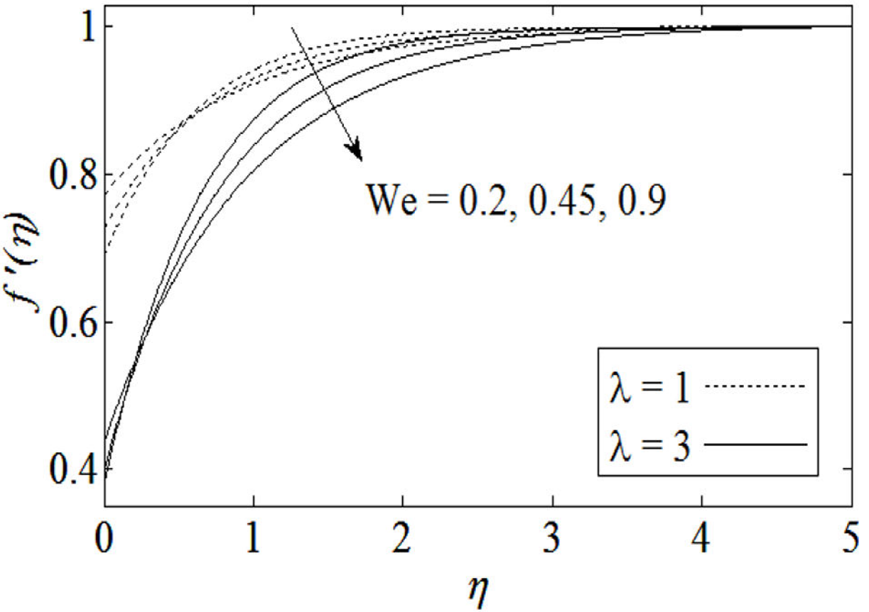
Figures 4 and 5 display the variation in f' and θ for various values of magnetic parameter M when Pr, β and We are fixed. The magnetic parameter can augment or suppress the velocity or it alters the boundary layer thickness. In the present case Fig. 4 illustrates that with an increment in M, the velocity is gained and momentum boundary layer thickness is reduced. According to Fig. 5, the temperature θ is diminished as the numerical value of M rises. A comparison of Figs. 3 and 5 suggests that effects of the magnetic parameter and slip on the temperature are the same. Therefore, following the same arguments the temperature shows a decrement with an increase in M. Furthermore, the thermal boundary layer thickness is reduced by increasing M. Variation in f' and θ for the influence of viscoelastic parameter We for fixed λ, M, β and Pr has been reported in Figs. 6 and 7.

Figure 6 shows that f' decreases by increasing We. This decrease in the velocity is due to increase in the effective viscosity of fluid for larger values of We. A reverse phenomenon has been observed near the surface as slip is increased. It means slip dominates the viscoelastic effects near the boundary. Temperature in this case is a decreasing function of We and results are shown in Fig. 7. To analyze the effects of β on f' and θ both for assisting and opposing flows, Figs. 8 and 9 are plotted. Figure 8 depicts that velocity f' is an increasing function of the mixed convection parameter β for the assisting flow and is decreasing function for the opposing flow. The reason is that when the fluid is in contact with the heated plate, the molecules of the fluid are excited and as a result the velocity of the fluid enhances. On the other hand, velocity of the fluid decreases near the cooled plate. Figure 9 shows the influence of β on the temperature θ. We observe that by increasing β the temperature of fluid reduces for assisting flow situation and it increases for the opposing flow. Impact of Pr on the numerical values of θ is displayed in Fig. 10. As expected temperature θ reduces for large values of Pr. From the explicit definition of Pr, we observe that it is inversely related to thermal diffusivity α. Therefore, increasing Pr, results in the decrement of α causing a decrease in heat transfer. This reduction becomes more prominent for the increased slip case.

Numerical values of skin friction coefficient f″(0) and local Nusselt number -θ'(0) for the influence of λ are presented in Table I both for assisting and opposing flow cases. It is observed that f″(0) is an increasing and -θ'(0) is a decreasing function of λ for the both cases. But magnitude of increase or decrease is smaller when there is an opposing flow. Table II is displayed for the analysis of f″(0) and -θ'(0) for the influence of magnetic parameter M. We see that by increasing M, both f″(0) and -θ'(0) gain the magnitude. The rate of increase of both quantities is larger in full slip regime and is smaller in no slip regime for both the cases. Effects of Pr on f″(0) and -θ'(0) on the lubricated surface has been depicted in Table III. The results show that by increasing Pr, f″(0) decreases and -θ'(0) increases in the case of assisting flow and both quantities accelerate in opposing flow situation. Table IV incorporates the effects of We on f″(0) and -θ'(0) during assisting and opposing flows for λ = 3, M = 1 and Pr = 1. We see that f″(0) and -θ'(0) are reduced by enhancing We in each case. Tables V and VI are presented to examine the variation in f″(0) and -θ'(0) for the influence of We, M and Pr. A comparison of obtained results for the no-slip case (λ = ∞) with those of Ahmed and Nazar ¹⁹ validates the accuracy of the provided solutions.

Table V. Comparison showing the influence various parameters on f″(0) when λ = ∞, for assisting as well as opposing flow situations. The numerical values written in the parentheses are calculated by ¹⁹ for the no-slip case. 

Table VI. Comparison showing the influence various parameters on -θ'0 when λ = ∞, for assisting as well as opposing flow situations. The numerical values written in the parentheses are calculated by ¹⁹ for the no-slip case. 

5. Conclusion

In this paper, effects of lubrication in MHD mixed convection stagnation point flow of a second grade fluid adjacent to a vertical plate has been investigated. A thin coating of a power-law fluid is used for the lubrication purpose. Numerical solutions are found to analyze the influence of slip parameter λ (ranging from no-slip to full slip), magnetic parameter M, Weissenberg number W _e , mixed convection parameter β and Prandtl number Pr on the flow characteristics. Results are presented in the form of tables and figures for certain values of parameters by considering assisting as well as opposing flow situations. Some findings of this study are

References

1. K. Hiemenz, Dingl. Poly-tech. 32 (1911) 321-410.
[ Links ]
2. K.R. Rajagopal, Journal of Non-Newtonian Fluid Mechanics 15 (1984) 239-246.
3. D.W. Beard, K. Walters, Proc. Camb. Phil. Soc. 60 (1964a) 667-674.
4. K.R. Rajagopal , T.Y. Na, A.S. Gupta, Rheol. Acta 23 (1984) 213-215.
5. K.R. Rajagopal , On boundary conditions for fluids of the differential type. In: Sequiera A. (Ed.). Navier-Stokes Equations and Related Non-Linear Problems. (New York, Plenum 1995).
6. K.R. Rajagopal , P.N. Kaloni, Some remarks on boundary conditions for flows of fluids of the differential type. In: Graham G.A.C. & Malik S.K. (Eds.). Continuum Mechanics and its Applications. (New York, Hemisphere, 1989).
7. A.C. Srivatsava, Z. Angew. Math. Phys. 9 (1958) 80-84.
8. G. Rajeswari, S.L. Rathna, Z. Angew. Math. Phys. (ZAMP) 13 (1962) 43-57.
9. D.W. Beard , K. Walters , Proc. Camb. Phil. Soc. 60 (1964b) 667-674.
10. V.K. Garg, K.R. Rajagopal , Mech. Res. Comm. 17 (1990) 415-421.
11. P.D. Ariel, Int. J. Eng. Sci. 40 (2002) 145-162.
12. M. Ayub, H. Zaman, M. Sajid, T. Hayat, Commun. Nonlinear Sci. Numer. Simulation 13 (2008) 1822-1835.
13. D. Li, F. Labropulu, I. Pop, Int. J. Non-linear Mech. 44 (2009) 1024-1030.
14. T. Hayat , Z. Abbas, I. Pop, Int. J. Heat Mass Transfer 51 (2008) 3200-3206.
15. M. Kumari, G. Nath, Int. J. Non-linear Mech. 44 (2009) 1048-1055.
16. M.M. Abdelkhalek, Int. Comm. Heat Mass Transfer 33 (2006) 249-258.
17. A. Ishak, R. Nazar, I. Pop , Comp. & Math. with Appl. 56 (2008) 3188-3194.
18. F.M. Ali, R. Nazar , N.M. Arifin, I. Pop , Journal of Heat Transfer 133 (2011) 022502-5.
19. K. Ahmad, R. Nazar , JQMA 6 (2010) 105-117.
20. F. Aman, A. Ishak , I. Pop , Appl. Math. Mech. Engl. Ed. 32 (2011) 1599-1606
21. B. Santra, B.S. Dandapat, H.I. Andersson, Acta Mechanica. 194 (2007) 1-10.
22. M. Sajid , K. Mahmood, Z. Abbas, Chin. Phys. Lett. 29 (2012) 024702.
23. P.A. Thompson, S.M. Troian, Nature 389 (1997) 360-362.
24. K. Mahmood , M. Sajid , N. Ali, ZNA 71 (2016) 273-280.
25. K. Mahmood , M. Sajid , N. Ali , T. Javed, International Journal of Physical Sciences 11 (2016) 96-103.
26. T. Cebeci, P. Bradshaw, Physical and Computational Aspects of Convective Heat Transfer. (Springer-Verlag. New York 1984).
27. H.B. Keller, T. Cebeci , AIAA Journal 10 (1972) 1193-1199.
28. H.B. Keller , A new difference scheme for parabolic problems, in Numerical Solution of Partial-Differential Equations (J. Bramble, ed.). Vol. II. (Academic, New York, 1970).
29. W. Ibrahim, B. Shanker, Computers and Fluids 70 (2012) 21-28.
30. D.D. Joseph, Boundary conditions for thin lubrication layer, Department of Aerospace Engineering and Mechanics, (1980) University of Minnesota, Minneapolis, Minnesota 55455.
text new page (beta)
English (pdf)
Article in xml format
Article references
Send this article by e-mail
Cited by SciELO