1. Introduction

The Γ(a,z) function is of most concern in the calculation of the temperature integral (TI) and it is closely related to both thermogravimetry (TGA)^1,2, and thermoluminescence dosimetry (TLD)^3,4. The TI integral has been approximated by several methods, mainly by asymptotic series^3,5 and continued fractions as the most sought-after^6,7. Likewise, a number of smart algebraic equations have also been proposed in order to approximate, analyze and compare the TI^8,9,10,11,12 from the fact that Γ(a,z) is a linear function. In some of these approximations, ranging from the least-squares fitting technique to a simple straight line (with respect to z), it is possible to obtain algebraic equations that accurately estimate the Γ(a,z) function^{11,13,14,15,16,17}. In this paper, some approximations by continued fractions to function Γ(a,z) and two for the particular case of a = -1are presented. These function approximations involve one to six fitting parameters, and show to have relative errors from 0.15% to 0.00042% within the interval 5≤Re(z)≤100. These approximations were obtained from a multidimensional least-squares fitting code NLREG. Considering the fast convergence of continued fractions and the straightforward evaluation of the algebraic expressions, the new reported approximants improve the calculation efficiency of the temperature integral. In this work, new approximations for the temperature integral, considering the fast convergence of continued fractions and the straightforward evaluation of the algebraic expressions are obtained. The new reported approximants improve the calculation efficiency of the temperature integral. The simplicity or precision of resent approximations, have a strong effect on values of physical quantities obtained from thermoluminescence data.

2. Basic equations

The upper incomplete gamma function Γ(a,z) is defined for z∈C, by

for all a with Re(z) > 0, and Re(a) < 0 if Re(z) = 0. This integral is of great importance in several areas of mathematical-physics surging along a diversity of contexts and applications, such as the application of Γ(a,z) in the analysis of the peaks shape in thermoluminescence dosimetry (TLD)¹.

Equation (1) can be written as

Where h(a, z) is defined as

The coupling of Eqs. (2) and (3) is carried out in a similar way by Chen and Liu¹⁶. Here, the multiplier z ^R is introduced (crucial in our methodology), and R is a real number. Equation (3) can be transformed to

and by differentiating Eq. (4) once in z, we obtain

Repeating several times this procedure, we obtain the n + 1order derivative in the form

where ξ=1+(R-a+1)/z. Noticing that the magnitude of the derivatives for h(a, z) is always lower than that for the function itself (for increasing n), we can approximate the left hand side of Eqs. (5) and (6) to zero. Thus, we obtain the solution of the n + 1-th equation which contains all the other lower order solutions, i.e., we obtain different approximations for h(a, z). From equation (5), and taking into account the first two equations from (6) we have

where the sub-index denotes the n-th order approximant. In Eqs. (7-9) as for all the system of equations (6), no restrictions are imposed to the value of R despite that in our case these values are just represented by continued fractions of the function h(a, z) (with different degree of approximation and complexity).

3. Numerical approximations to Γ(a,z) with real z

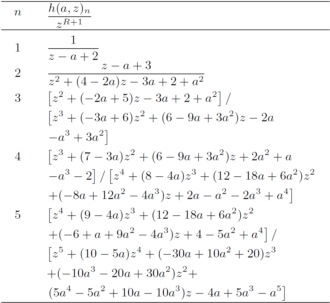
In this section we show a family of continued fractions that approximate the Γ(a,z) function. Among the whole set of rational fractions for h(a, z) there are four subsets characterized by their simplicity of a continued fraction. Three of them are obtained for R = -1, 0, 1 (Tables I to III).

Table I. Rational fractions for h(a, z) _n /z ^R+1 obtained with R = -1. 

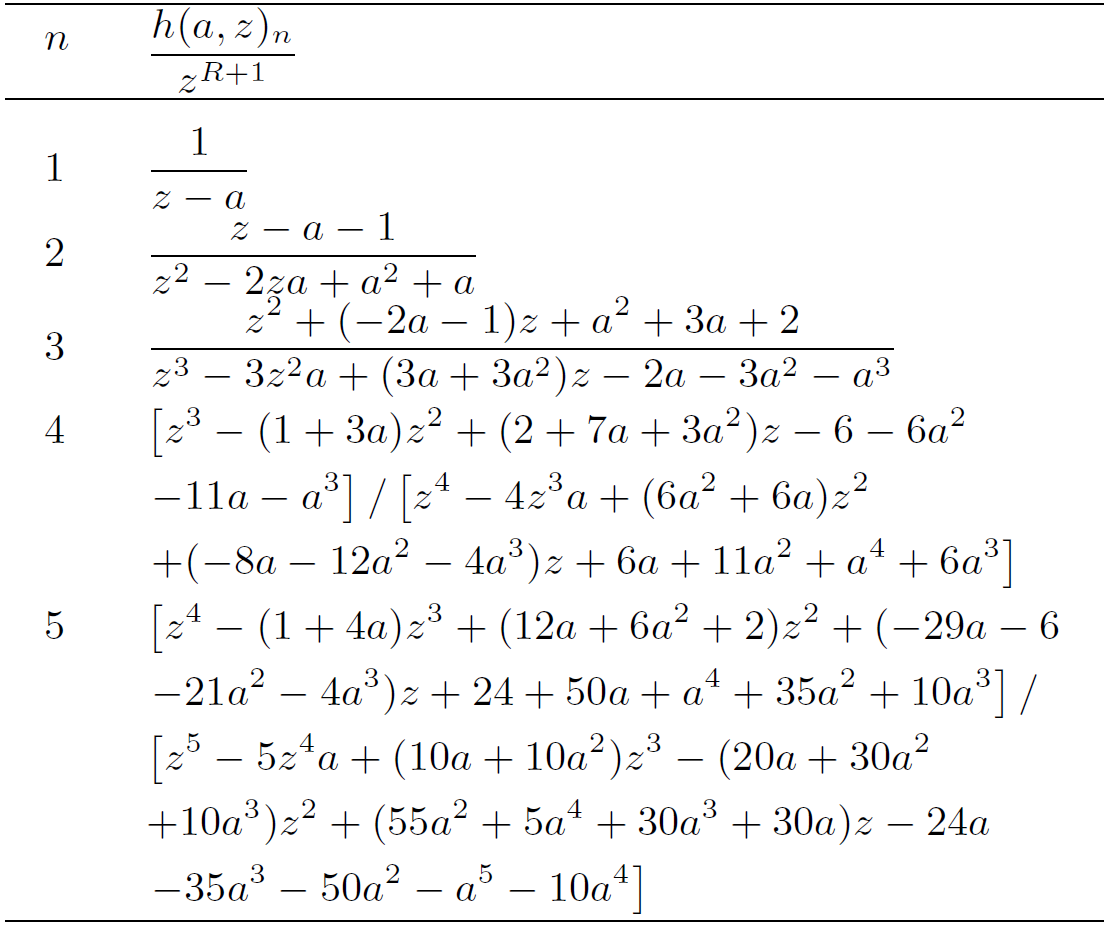
Table II. Rational fractions for h(a, z) _n /z ^R+1 obtained with R = 0. 

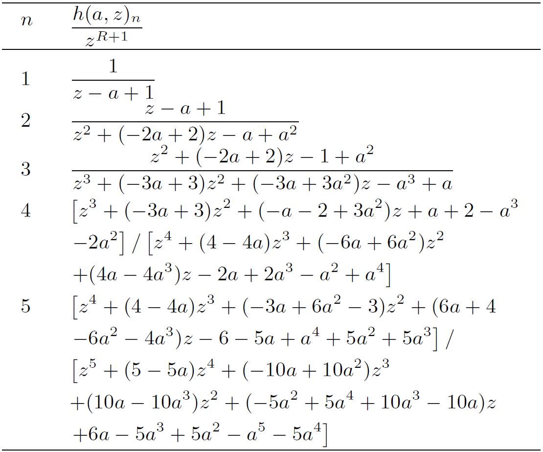
Table III. Rational fractions for h(a, z) _n /z ^R+1 obtained with R = 1. 

One representation by continued fractions of Γ(a,z) is obtained for R = -1 in the form (we adopt the notation introduced in Ref. 18)

Similarly, the rational fractions for R = 0,1 and n≥2 respectively, can be put together in a similar way as in Eqn. (10) to obtain,

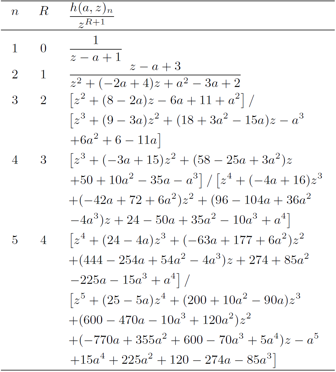
The other one arises from the combination of n and R values, respectively. Substituting the continued fractions for h(a, z), obtained from the first five rational fractions with a set of pairs {n,R}={1,…,5;0,…,4} (Table IV), into Eq. (2) we get the Γ(a,z) function in the form¹⁸

Table IV. Rational fractions for h(a, z) _n /z ^R+1 obtained for n = 1 … 5 and R = 0 … 4. 

Expression (13) is the well-known representation by continued fractions of Γ(a,z) reported in textbooks⁵. Equation (13) was applied to thermoluminescence dosimetry in Refs. ¹⁹ and ²⁰. All these arrangements of rational fractions by continued ones, Eqs. (10-13), were obtained from the “confrac" Maple function²¹.

The relative truncation errors of Eq. (13) assuming a real z, is resumed in Table (V), where the relative truncation error is defined as

here n corresponds to the n-th approximant and F (a, z) is the full approximation to Γ(a,z).

Table V. Relative truncation errors for the first 20 approximants in Γa, z for a = 1/2 from the most rapidly convergent expansion (13). 

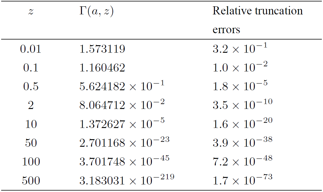
The evaluation of the special function for the selected arguments is rounded to exact seven decimal digits and the truncation errors are upward rounded to 2 decimal digits. Equations (11-12) are the standard approximations to the gamma function and Eq. (10) becomes the least accurate approximation to the Γ(a,z) function. However, all approximations can be useful in several applications abroad, e.g. in the calculation of the thermoluminescence line shape²² where only the real values of z > 5 with accuracy of up to two or three significant figures of merit are needed. Therefore, continued fractions Eqs. (10-13) can be employed with up to five approximants. Another criterion used to compare several approximations for Γ(a,z) is the maximal relative error given by

This criterion will be used in the following, as well as the assumption of a real z.

4. Two simple approximations for a real z

In order to simplify the first three approximants of continued fraction, Eq. (13), we account for the fact that the polynomial order in the numerator is less that one as compared to the order in the denominator. In this sense, we look for a ratio of polynomials of order (n-1)/n in the form

or

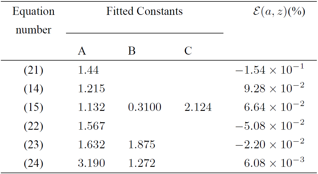
where A, B and C are the parameters to be fitted. The rational approximations on the right hand side of Eqs. (14-15) have been taken as test functions in the least-squares fitting, looking for the minimal number of coefficients to be fitted. The least-squares fitting using the NLREG code²³, gives the parameters A, B and C accounting for the set of values a={-4,-3,-2,-1, 0, 1, 2} and z={5, 6, 7,⋯,100} resulting in 576 points. The fitted values are summarized in Table VI. The Eq. (14) has the peculiarity of using a single fitting parameter.

Table VI. Fitted parameters and their maximal relative error E(a,z) for proposed approximations. 

Now, we obtain better approximations as compared to Eqs. (14) and (15). Equation (9) with n = 2, as a continued fraction takes the form,

Introducing the quantity γ=z-a+1 in Eq. (16), this results in

Expanding the denominator in Eqn. (17) into a binomial series and conserving only the first two terms, we have

Equation (18) is valid for a∈(-4,1/2) and z≫1 and can be simplified, for example, by factorizing the γ variable in the denominator of the second term in brackets and expanding into binomial series, we get

Finally, turning back the value of γ=z-a+1 in (19) we obtain

In Eq. (19), the constant number γ in the denominator in brackets on the right hand side becomes the unique free variable. Thus, intuitively we can choose the following approximations forward that maintain the structure of Eq. (19)

where A, B, C and E(a,z) in Eqs. (21-24) are the parameters determined by a bi-dimensional least-squares fitting with respect to a and z (summarized in Table VI). In case of the Eq. (25), we obtain A = 1.7256, B = 1.3219, C = 0.29606, D = -3.0279, E = 3.6887, F = 0.51297 and E(a,z)(%)=4.16×10-4.

The fitting is carried out, as previously, comparing the left hand side of Eqs. (21-25) for several values of a and z with test functions as on the right hand side. From the fitted results, we observe that the more complicated the test functions the approximations result better.

5. Comparison with other published approximations with a real z

The generalized temperature integral is defined as²⁴,

There are several algebraic expressions that approximate Eq. (26) using the Γ(a,z) function. To show the close relation between Eq. (26) and the Γ(a,z) function, we make m = -a - 1 in (1), and obtain the relation

Six reported approximations for the Γ(a,z) function are given by^{13,14,16,17,25}

Where A, B, C, D, E and F in Eqs. (28-32) are the fitted parameters, summarized in Table VII.

Table VII. Values for fitted parameters in approximation Eqs. (28-32) for the Γ(a,z) function and their maximal relative error E(a,z). 

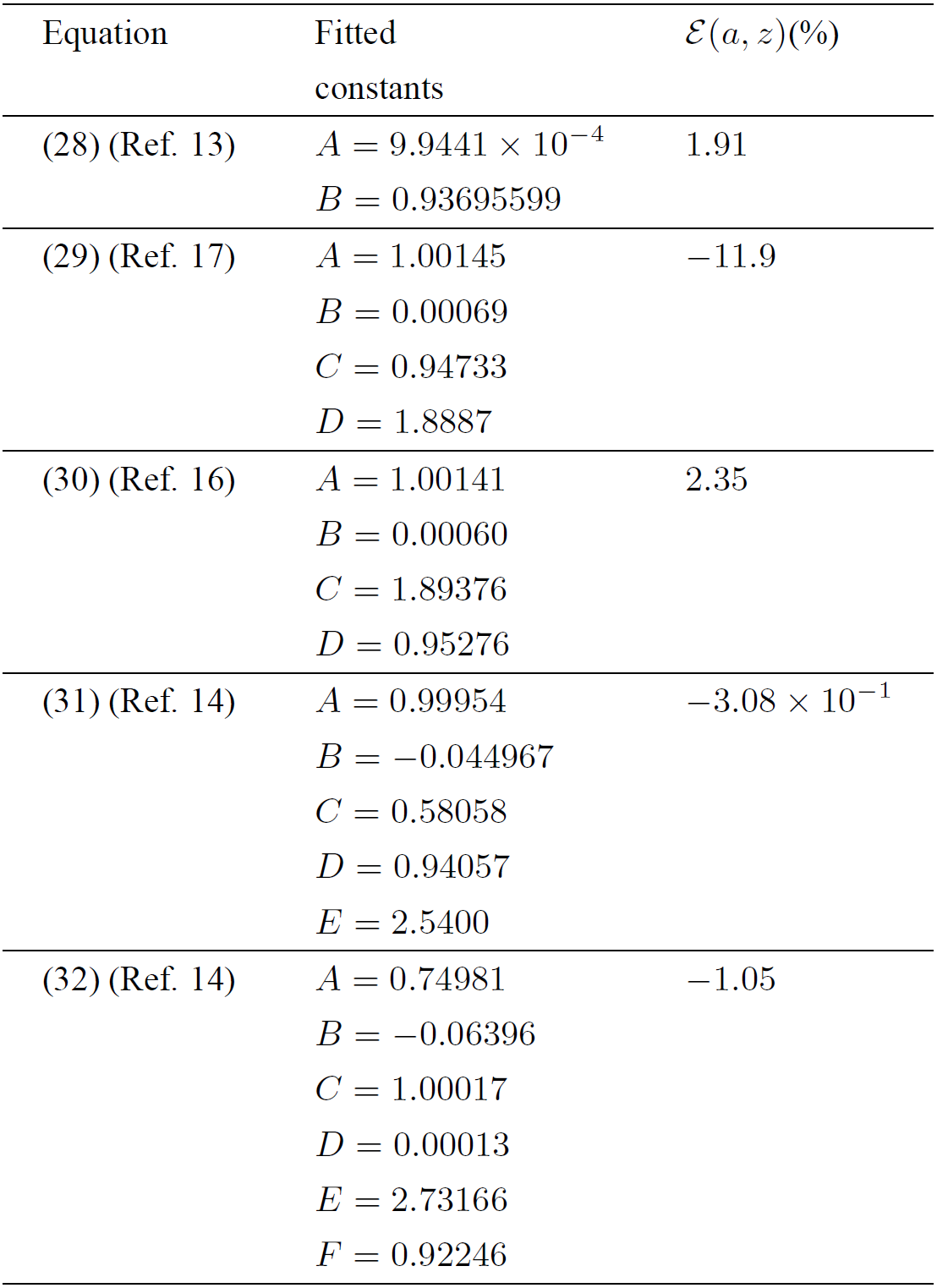
From the comparison of the values for maximal relative errors from the proposed (Table VI) and reported approximations (Table VII), we note that for those proposed ones the error becomes smaller.

6. Case of the temperature integral for Arrhenius equation (a = -1, m = 0)

An important particular case, for the Γ(a,z) function, is the value a = -1 in the fourth approximant (n = 4) of continued fraction Eq. (13),

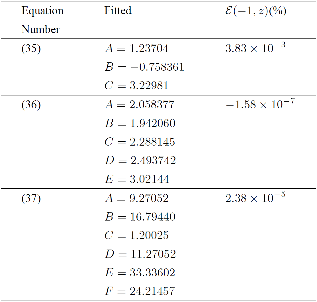
This equation represents the Senum and Yang approximation⁸ used as a test function by several authors^9,12. The maximal relative errors for the cases of Eqs. (24), (25), (34) (n = 4) and (13) (n = 10) are E(-1,z)={-4.88×10-3,3.52×10-4,3.13×10-3,2.5×10-7}, respectively. A similar maximal relative error as for Eq. (34) is obtained in case of the simpler approximation a = -1 from Eq. (15), written in the form

where A = 1.132, B = -0.620 and C = 3.124. Considering these values as the initial ones in a least-squares fitting to synthetic generated data from the left hand side of Eq. (35) on a set of points z={5, 6, 7,⋯,100} we find those values for A, B and C summarized in Table VIII. In order to reduce the maximal relative error of Eq. (24) and Eq. (25), in a one-dimensional least-squares fitting, we propose the next test expression

Table VIII. Values for fitted parameters and the maximal relative error for the case a = -1 evaluated in the interval z={5, 6, 7,⋯,100} and their maximal relative error E(a,z). 

to determine the parameters A, B, C, D and E (Table VIII). This test equation is compared to that equation proposed in Ref. 12, in the form

where the values for their corresponding parameters are summarized also in Table VIII. Comparing the maximal relative errors of Eq. (36) and Eq. (37), we observe that approximation Eq. (36) containing only five fitting parameters, not six as in Eq. (37), reduces the error in two orders of magnitude.

We can observe that it is a compromise between the minimal error reached and the simplicity of the approximation. Thus, expressions systematically obtained from the continued fractions method, show that these two properties could be rather simple or become complicated as needed for numerical calculations.

7. Conclusions

New modifications that approximate the incomplete gamma function Γ(a,z) are presented. All these fractions are compared by the maximal relative error E(a,z) for a wide range of values for the argument 5≤R(z)≤100. All approximations obtained become highly useful for the particular case of thermoluminescence line shape calculation and the most important fact: they are valid for all values of z, a required condition in experimental data analysis. The expressions obtained for the TI could be incorporated in glow deconvolution line treated by different methods such as in the project GLOCANIN²⁶ and the TGCD package²⁷. Thus, expressions systematically obtained from the continued fractions method, show an equilibrium between the minimal error reached and the simplicity of approximations, and could be simple or complicated as needed for numerical calculations.

References

1. G. Gyulai and E.J. Greenhow, J. Therm. Anal. 6 (1974) 279-291.
[ Links ]
2. A. Mianowski, J. Therm. Anal. Cal. 60 (2000) 79-83.
3. Y.S. Horowitz and D. Yossian, Radiat. Prot. Dosimetry. 60 (1995) 1-114.
4. C. Furetta, Handbook of thermoluminescence, (World Scientific, Singapore, 2003).
5. M. Abramowitz and I.A. Stegun, Handbook of Mathematical Functions with Formulas, Graphs, and Mathematical Tables (National Bureau Standards, Washington, 1970) pp. 253-293.
6. W.L. Patterson, J. Comp. Phys. 7 (1971) 187-190.
7. S.D. Singh, W.G. Devi, A.K. Singh, M. Bhattacharya, and P.S. Mazumdar, J. Therm. Anal. Cal. 61 (2000) 1013-1018.
8. G. Senum and R.T. Yang, J. Therm. Anal. 11 (1977) 445-447.
9. L.A. Pérez-Maqueda and J.M. Criado, J. Therm. Anal. Cal. 60 (2000) 909-915.
10. V. Rao and M. Bardon, J. Therm. Anal. 46 (1996) 323-326.
11. T. Wanjun, L. Yuwen, Z. Hen, W. Zhiyong, , and W. Cunxin, J. Therm. Anal. Cal. 74 (2003) 309-315.
12. L.Q. Ji, Therm. Anal. Cal. 91 (2008) 885-889.
13. T. Wanjun, L. Yuwen, Y. Xil, W. Zhiyong, and W. Cunxin, J. Therm. Anal. Cal. 81 (2005) 347-349.
14. J.M. Cai and R.H. Liu, J. Therm. Anal. Cal. 90 (2007) 469-474.
15. H.X. Chen and N.A. Liu, J. Therm. Anal. Cal. 92 (2008) 573-578.
16. H.X. Chen and N.A. Liu, J. Therm. Anal. Cal. 90 (2007) 449-452.
17. T. Wanjun and C. Donghua, J. Therm. Anal. Cal. 98 (2009) 437-440.
18. A. Cuyt, V.B. Petersen, B. Verdonk, H. Waadeland, and W.B. Jones, Handbook of continued fractions for special functions, (Springer, Netherlands, 2008) pp. 238-244.
19. H. Flores-Llamas and C. Gutiérrez-Tapia, Radiation Effects and Defects in Solids 168 (2013) 48-60.
20. P.R. González, C. Gutiérrez-Tapia, and H. Flores-Llamas, Appl. Rad. Isotopes 83 (2014) 200-203.
21. Maple 16.02, http://www.maplesoft.com (2012).
22. M. Bhattacharya, N.C. Deb, A.Z. Msezane, , and P.S. Mazumdar, Phys. Stat. Sol. (a) 185 (2001) 291-299.
23. P.H. Sherrod, Nlreg nonlinear regression analysis program v. 6.3," http://www.nlreg.com (1991).
24. I. Agherghinei, J. Therm. Anal. 36 (1990) 473-479.
25. J.M.V. Capela, M.V. Capela, and C.A. Ribeiro, J. Therm. Anal. Cal. 97 (2009) 521-524.
26. A.J.J. Bos, T.M. Piters, J.M.G. Ros, and A. Delgado, Radiat. Prot. Dosim. 51 (1994) 257-264.
27. J. Peng et al., Thermoluminescence glow curve deconvolution: Package “tgcd” v. 1.7, (2015). http://CRAN.R-project.org/package=tgcd
text new page (beta)
English (pdf)
Article in xml format
Article references
Send this article by e-mail
Cited by SciELO