


 text new page (beta)
 English (pdf)
 Article in xml format
 Article references
 Send this article by e-mail
 Cited by SciELO
  Similars in
SciELO
Similars in
SciELO 
 Permalink
PACS: 42.68.Wt; 42.79.Qx
1. Introduction
Atmosphere and weather have become a topic of great concern not only for scientists but for many people. Terms such as greenhouse effect, ozone depletion and global climate change are words that are now used routinely as an indication of that concern. A key activity to understand the behavior of the atmosphere is the ability to know its structure, making it necessary to develop suitable measurement systems to resolve the spatial and temporal variation of the atmospheric structure and composition.
Remote sensing techniques with potential application for studying the atmosphere started in the first half of the last century. During World War II systems such as Radar (radio detection and ranging) and Sonar (sound navigation and ranging), were developed for the detection and ranging of aircraft or as a navigation tool for submarines. Whereas radar is based on the emission and detection of an electromagnetic pulse in the atmosphere, sonar is based on the emission and detection of underwater acoustic pulses.
The idea of studying the atmosphere with light sources dates back to 1930 when Synge1 and a group of scientists first suggested the use of intense light sources to estimate the density of the atmosphere. The first such experiments were reported in 1937 by Hulburt2 and years later by Elterman3 in 1954. After the invention of the ruby laser by Maiman4 in 1960, McClung and Hellwarth5 reported for the first time, in 1962, the propagation and scattering of laser light in the atmosphere. The first formal application in the study of the atmosphere was carried out by Fiocco and Smullin6 of the Massachusetts Institute of Technology (MIT) who in 1963 reported laser-light echoes from the troposphere and the upper regions of the atmosphere. The same year, Ligda7 used the first lidar techniques for tracking volcanic particles in the troposphere; from these studies, the lidar started to be widely recognized. It is likely that the term lidar (light detection and ranging) to describe this new laser tool was coined by Collis and Ligda8,9 in 1966.
Lidar is based on exactly the same principle in which radar is based; the only difference is that in the former, the radiation emitted is in the range of frequencies close to those of visible light. Nowadays, the discovery of new laser sources, the development of new compounds and materials, advances in optics, optoelectronics, detectors, electronic systems for data acquisition and signal processing, have enabled the exploitation of the potential of lidar in an extraordinary variety of atmospheric applications.
2. A Brief History of Lidar in Mexico
In the late 70s, while in some industrialized countries like Canada, France, Italy, United Kingdom and United States there existed full momentum in the development of lidars of different types and applications, in Mexico there was no activity related to this subject. Lately, in 1986, as part of a scientific cooperation between the governments of Mexico and Italy, a joint development of a Differential Absorption Lidar (DIAL) suitable to detect sulphur dioxide (SO2) in the atmosphere was agreed. The main objective of this project was to transfer lidar technology to Mexico, in which Italian scientists had vast experience as they had successfully developed DIAL systems for detection of SO2, nitrogen dioxide (NO2), ozone (O3) and other airborne compounds. The DIAL would be jointly developed by researchers at the Centro Informazione Studi Esperienze (CISE) in Italy and by researchers of the Electrical Research Institute (IIE) in Mexico. In 1989 the DIAL system was officially commissioned in Mexico. Since then, measurements of SO2 in atmosphere were performed at several power stations such as: Petacalco, Tula, Valle de Mexico, Manzanillo, Jorge Luque; the Atzcapotzalco petroleum refinery, and industries such as Colgate-Palmolive, among others.
Having developed an actual interest in lidar technology, during the late 90s a small group of researchers at the IIE began a project to develop an elastic-scattering lidar in order to complement the research that was performed with the DIAL in studies on the structure of the atmosphere. The project was suspended and resumed several times. It also faced many difficulties such as scarcity of resources and policy changes within the IIE. Finally, and despite these difficulties, this group of researchers managed to complete an early prototype whose tests yielded favorable results10.
A few years later, a group of researchers including one member of the original pioneers in Mexico, some of them based at the National Institute of Astrophysics Optics and Electronics (INAOE for its acronym in Spanish), has taken up the initiative to continue the development of lidar systems, especially the elastic-scattering lidar, which is now completed and described in this work.
3. The lidar
In a general scheme, a lidar can be classified, depending on the interaction that the laser light suffers with the atmosphere, into two categories: elastic-scattering lidar and inelastic-scattering lidar. In the first kind are included the phenomena in which the laser radiation is scattered by atoms, molecules, aerosols or particles in the air, without undergoing a change in its wavelength (or frequency). On the other hand, in inelastic scattering, a change in the wavelength of the scattered radiation exists, i.e. the frequency (or energy) of the incident photon is different from the frequency of the scattered photon. Here, within these techniques, the Raman lidar11 and the fluorescence lidar12 can be mentioned.
The operational principle of the elastic-scattering lidar (or simply elastic lidar) is based upon the elastic scattering that the laser light suffers as it propagates through the atmosphere. As mentioned above, the elastic term refers to the scattering and returning of light at the same wavelength as that emitted by the laser. The light scatterers are the particles and gases that constitute the atmosphere present throughout the propagation path of the laser beam.
An elastic lidar does not detect the presence of a compound or chemical species individually, but the bulk scattering produced jointly by the presence of these gases, compounds, particles and aerosols in the atmosphere. This allows the localization, in direction and range, of zones in which changes of the atmospheric structure exist such as: gradients of density, humidity, dust, mixing layer, pollutant plumes, etc.
4. Description of the elastic-lidar
The developed lidar and its components are illustrated in the diagram of Fig. 1. An intense and very short pulse of light is generated by the Nd:YAG laser and directed, through the output optics, towards the atmosphere. A 50 mm Galilean beam expander with expanding factor of 25 (suitable for 532 nm) was used to reduce the intensity and dangerousness (not the energy) and also to reduce the divergence of the laser beam to less than 0.4 mrad. For the sake of safety, a “panic button” is incorporated into the lidar system, which allows the immediate shutdown of the laser in case of any human or fauna activity in the sky within the scanned region/area (airplanes, birds, etc.).
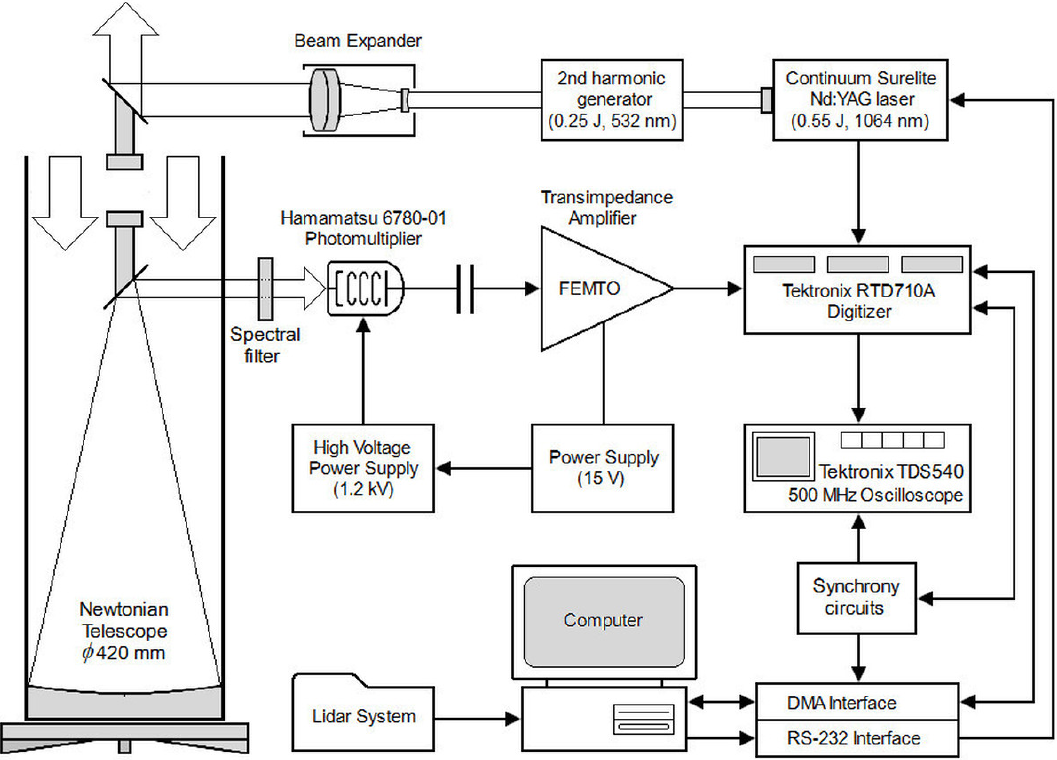
The scattered radiation that returns backward to its origin point (phenomenon known as backscattering) is collected and focused by the telescope (through the spectral filter) to the Hamamatsu photomultiplier. The spectral filter distinguishes the laser light from the background radiation such as diffuse solar or artificial light at other wavelengths. The luminous signal at the photomultiplier is then converted into a voltage signal by a low-noise transimpedance amplifier. This analogue voltage signal, or ‘return signal’, is transferred to the Tektronix digitizer where is converted into numerical data that can be processed or stored in a computer for further analysis. The analogue signal can be monitored with the oscilloscope in order to observe the behavior of the received signal. Since the luminous signal is acquired in real time and the phenomenon occurs at short time scales, it must be acquired with high-speed electronics.
The return signal power of an elastic-scattering lidar is described by the well-known classic equation13,14.
where, P
L
is the power of the laser source; c is the speed of light;
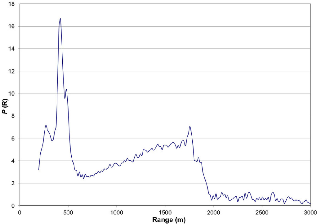
Figure 2 shows a graph of an actual lidar return signal. Essentially, it is a plot of the radiative power of the received backscattered light as a function of range. As can be noticed, any non-homogeneity in the atmosphere, together with its distance and direction, is revealed by the local intensity of the backscattered signal.
5. The elastic-lidar signal processing
In order to process the elastic-lidar signals, the authors have developed a simple mathematical procedure based on the lidar equation. This methodology highlights the gradients of the atmospheric backscattering properties by calculating the relative backscattering coefficient. The method has been tested experimentally in real cases with satisfactory results14.
According to Eq. (1) and assuming that another backscattering element is located at range
then the ratio between the scattered power from range R and the scattered power from R + L can be written:
The variable L is the spatial resolution of the system, whose length is defined by the rate at which the digitizer samples and digitizes two consecutive points of the lidar return signal.
Since the receiver optics and the laser are arranged coaxially and the field of view of the optical setup is greater than the area irradiated by the laser, it is clear that for every R:
Therefore,
Then, considering that the coefficient
Finally,
where constant
Equation 7 describes the relative backscattering coefficient of atmospheric elements located along the laser pulse traveling in an atmosphere with constant density. However, most lidar measurements are carried out in the zenithal direction, where the air density decreases with altitude, having an effect on the measurements and therefore in the processing of the return signals. This effect can be taken into account by extending Eq. 7 as follows.
The atmospheric air pressure with respect to the altitude can be estimated through the hydrostatic equation15:
where p is the atmospheric pressure,
where
At low altitudes (z
and with Eq. 9:
Substituting the values of the constants, and considering
At ground level in Cuernavaca city, z = 0:
let the constant h be:
Eq. 7 then becomes:
This final expression is used for processing the lidar signal data specifically for zenithal probing of the atmosphere over the Cuernavaca city, México.
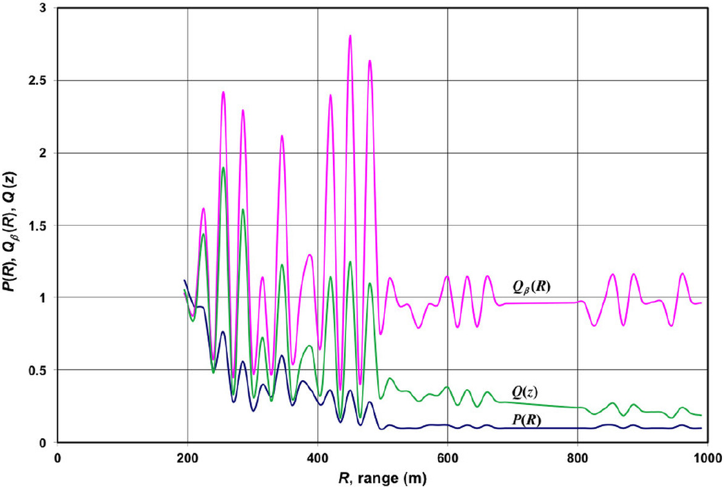
The plots
6. Experimental testing and results
The elastic-scattering lidar was tested in probing of the atmosphere in the city of Cuernavaca, Mexico. The measurements were carried out with a Q-switched Nd:YAG laser (made by Continuum®) with a second harmonic generator at a wavelength of 532 nm and stabilized in frequency to a linewidth of 300 MHz and an energy of 250 mJ per pulse (at 532 nm)17. The laser was firing at 20 Hz and the scattered light was collected with a 420 mm diameter telescope. The lidar return signals were sampled with a Tektronix® digitizer which high acquisition speeds resulted in a spatial resolution of L = 15 m. Each post-processed signal represented the average of over 25 laser firings. In order to better present the results, the data were plotted in a 3D (x, y, color) plot with the software Python®.
The figures shown below correspond to results obtained by zenithal lidar probing of the atmosphere above the city of Cuernavaca that was carried out at the facilities of the Electrical Research Institute (IIE), located at: 18.875770°N; 99.219477°W.
Figures 4 and 5 are plots of zenithal height-time scans to an altitude of 3,000 m. Figure 4 clearly shows the stratified layers often found during very stable atmospheric conditions. As can be noted a layer containing high concentration of particulates is shown at an altitude of 500 m. Above 2,000 m a clear atmosphere is visible. Figure 5 shows that most of the particulate concentration is below an altitude of 700 m, which probably indicates an atmospheric thermal inversion event. A clear atmosphere above 1,500 m is distinctively observed.
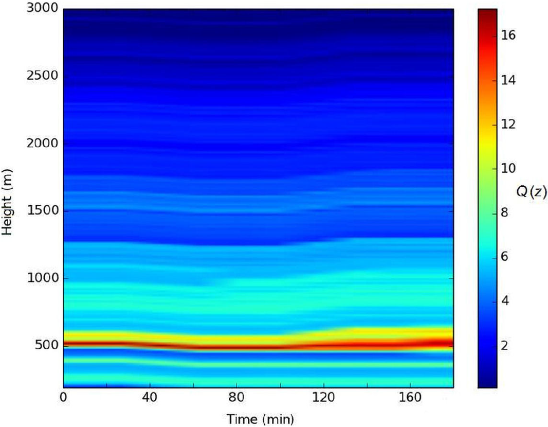
Figure 4. A plot of a long range height-time scan obtained over the city of Cuernavaca at 8:30 a.m. local time, December 11th, 2012.
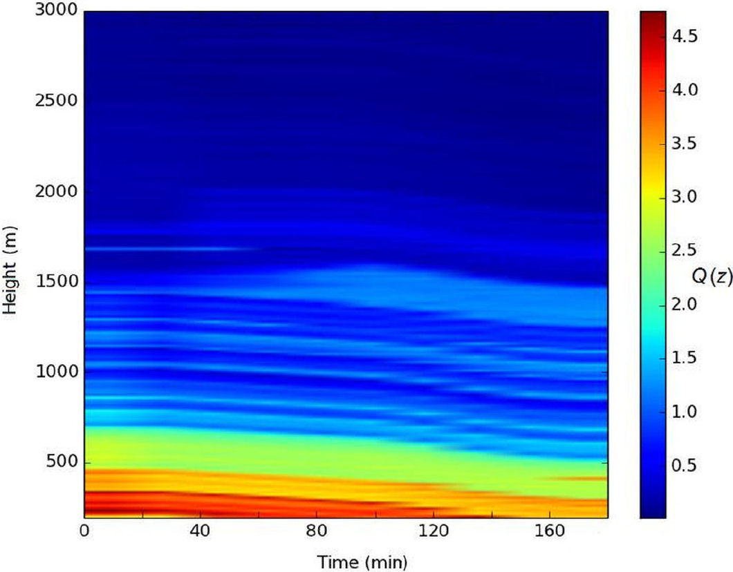
Figure 5. A plot of a long range height-time scan obtained over the city of Cuernavaca at 8:30 a.m. local time in December 12th, 2012.
Figures 6 and 7 are plots of zenithal height-time scans performed to an altitude of 1,000 m. Figure 6 shows a big moving mass of air with a high concentration of particulates.

Figure 6. A plot of a medium range height-time scan obtained over the city of Cuernavaca at 12:00 p.m. local time, January 18th, 2013.
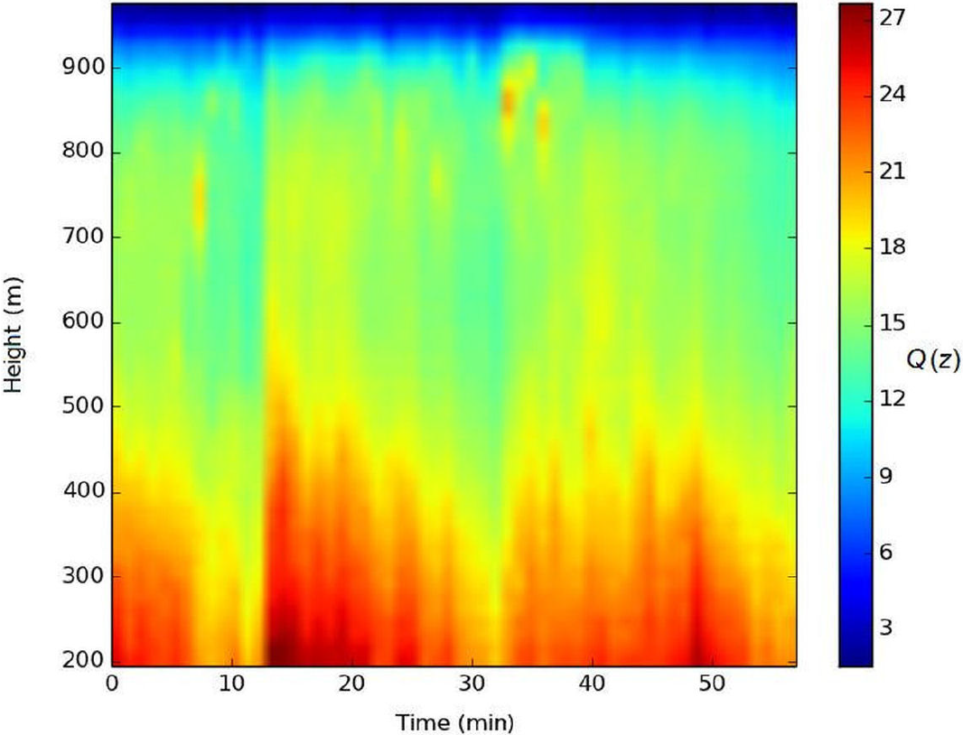
Figure 7. A plot of a medium range height-time scan obtained over the city of Cuernavaca at 12:30 p.m. local time, January 20th, 2013.
Figure 7 is a very interesting example, which shows periodic instabilities in an atmospheric path with a high concentration of particulates. Authors such as Einaudi18 refer to these periodical instabilities as atmospheric ‘gravity waves’ because they are oscillations caused by convection forces between cold and warm air parcels. As noted, gravity waves are only developing at an altitude below 900 m; at higher elevations, a clear and very stable atmosphere is shown.
7. Conclusions
The development and testing of an elastic-scattering lidar has been presented in this work. The lidars capability to reveal the profile of the atmospheric structure in the zenithal direction was used to determine the height and thickness of atmospheric layers or strata, as well as their spatial and temporal evolution.
Moreover, the authors have developed a simple method that allows the processing of the elastic-lidar return signals, thereby providing the details of the atmospheric structure being probed. It is essential to draw attention to the capabilities of this method to uncover hidden or masked details in the raw lidar signal. Furthermore its ability to extract information on the shape and location of the atmospheric features in heavily polluted atmospheres has also been demonstrated. The cases described in this manuscript clearly demonstrate the effectiveness of the proposed method.
The authors wished to share their experience of the construction of a lidar system together with the development of a simple, but powerful processing method that has the potential to be further improved. We believe that this modest contribution could help with the design and use of cutting edge lidar systems in Mexico with important applications such as air quality monitoring and/or the measurement of the transport and evolution of pollutant plumes produced by factories or volcanoes, among others.

