


 nueva página del texto (beta)
 Inglés (pdf)
 Artículo en XML
 Referencias del artículo
 Enviar artículo por email
 Citado por SciELO
  Similares en
SciELO
Similares en
SciELO 
 Permalink
PACS: 05.45.Df; 05.10.-a
1. Introduction
The term “fractal" defines irregular, rough or complicated shapes that cannot be described by the Euclidean geometry1. The fractal dimension, D, can be defined as a measure of the complexity or roughness of this kind of shapes and can be treated as the degree to which a set “fills" the Euclidean space in which it is embedded2. Due to the above mentioned properties the value of D is fractional. The fractal dimension has a large number of applications in different areas of science and engineering, such as: modeling of forest fires3, flow in porous media4, imbibition in disorder media5, percolation6, electroosmotic in porous media7, which can have scaling behavior of self-avoiding walks8. In many of these cases, it is necessary to estimate the fractal dimension of bitmap images of rough self-avoiding curves embedded in
In practice, the estimation of fractal dimension of a rough interface from an image is challenging12 and there are two types of procedures for the estimation. The first type is implemented with the use of estimators (graphical) that operate binary images of interfaces and estimate D directly. For example, software Benoit 1.313 and FracLac14 perform such routines based on the Box-count1 estimations, among others. In the second kind of procedures the binary image of a roughened interface, which can be represented as a self-avoiding walk8, is transformed into a single-valued series, and the estimation of D is performed using the numerical information from this transformed profile4 choosing an adequate estimator for time series. This kind of methods results in a modification of profile information due to the cutting or filling of the ridges and valleys formed, which leads to an error in the estimation of the fractal dimension of the original interface profile (an example of this procedure is presented below in the Sec. 3).
In this work we demonstrate that both kinds of actual methods do not provide reliable estimates for self-avoiding profiles. The aim of the work is the development of a novel method of estimation of fractal dimension D based on the generalization of the estimators of Box-count and Hall-Wood for self-avoiding rough interfaces embedded in
2. Methods of fractal dimension estimation
Essentially, all the methods designed for the estimation of D are based on a common scheme in which D is induced as a function of scale governed by a power law and the estimate is obtained using a linear regression fit with least squares method. It should be noted that not all the estimators are applicable to the same kind of data15, therefore in order to obtain a reliable estimate it is necessary to perform a careful choice of estimation method in dependence on the data type and its representation (statistical data series or image).
2.1 Box-count estimator
Box-count estimator is one of the most popular and commonly used estimators, and it is motivated by the following scaling law:
where D
BC
is the Box-counting dimension,
i.e. graph of time series or spatial data X
t
observed at finite time set
The main idea of this method is that initially the series graph is covered by a single bounding box, which is divided in four quadrants. This process is repeated subsequently with each of the quadrants until the resulting box width matches the resolution of the data recording the number of boxes required at each step. Thus, if
Some authors identified problems with the original Box-count estimator, which includes all scales in the least squares regression fit of
2.2 Hall-Wood estimator
Peter Hall y Andrew Wood16 introduced a Box-count estimator modification for fractal dimension D
HW
, which operates to the smallest observable scales. Let
which results in a reformulation of definition (1) being:
On scale
This estimator has better accuracy as compared to the original method of Box-count 15, but its disadvantage is that it can only be applied to the case in which the set of points X is a single-valued profile (interface) of form (2), that is, the time series graph or spatial data observable on a finite set
2.3 Madogram and Variogram estimators
In the case when the data is given as a time series data or spatial data observed on a finite set
If
where
where
The Variogram estimator is obtained using the classical method of moments estimator for
For p = 1, is more efficient and the relation (5) between the fractal dimension D and the fractal index
Generally, the lower is the value of roughness exponent
3. Results
To compare the efficiency of common methods of fractal dimension estimation of both kinds (graphical and statistical) the degrees of variation of the estimates obtained by the both kinds of estimators were investigated. For this aim, synthetic samples data series with a known D value were generated in MatLab18. All the samples had 1500 fractional values and were divided into three groups, with the D values of 1.2, 1.5, and 1.8. Thereafter the fractal dimensions of the data samples were numerically estimated by fractaldim package19, using Box-count, Hall-Wood and Variogram statistical estimators. Furthermore, the data samples were also transformed in graphical bitmaps, binarizing the image, and after that their fractal dimensions were estimated using the fractaldim package in the same procedure for the data essays.
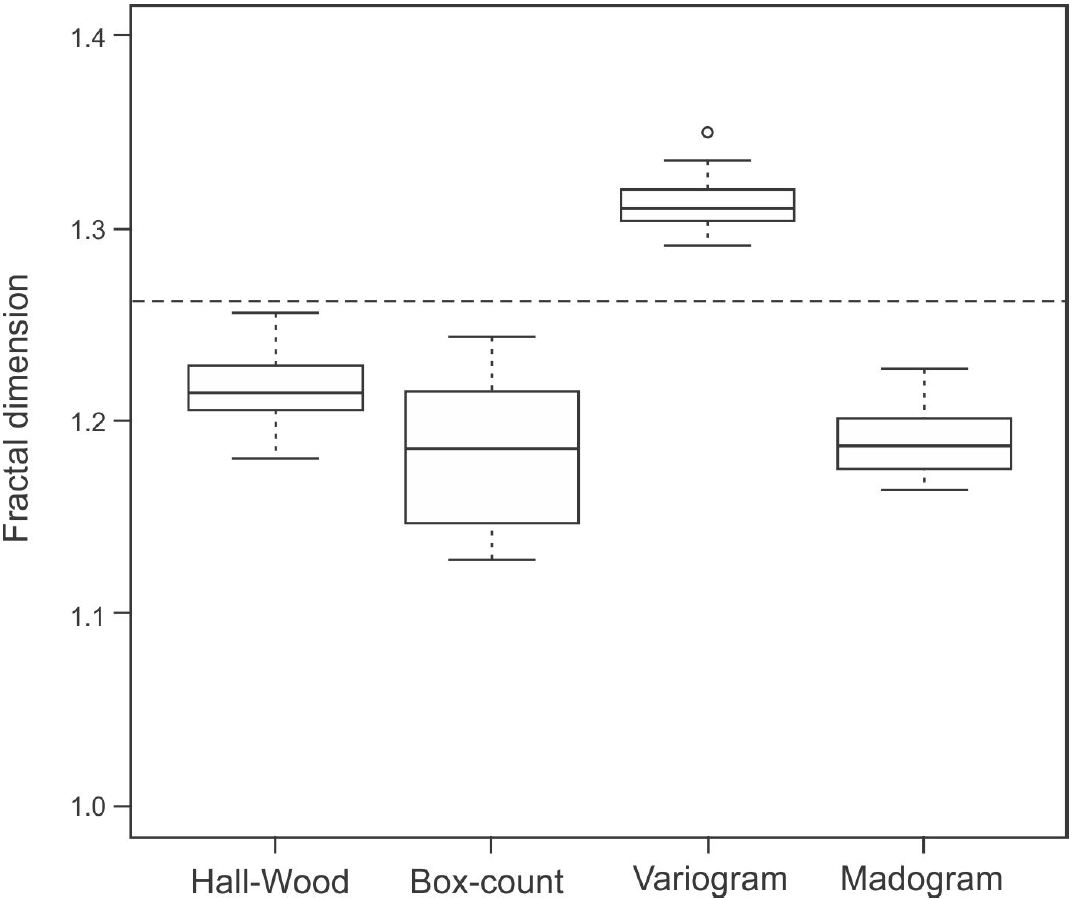
The results of the estimates from the two sources of information (data series and graphical bitmaps) of the samples were compared. In Fig. 1 the mean variances obtained for the 4500 samples of both kinds of estimators are shown.
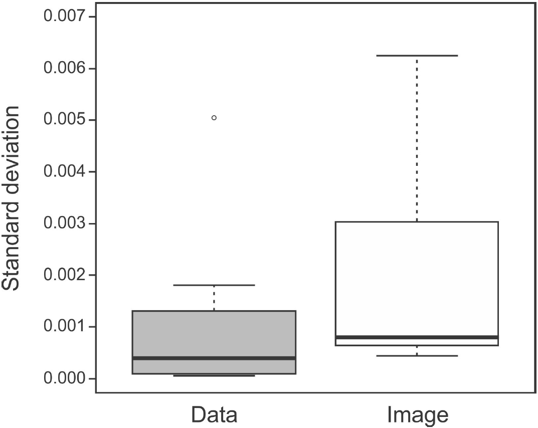
Figure 1. Comparison of standard deviations of estimates for same data series obtained by two types of estimators: graphical (image) and statistical (data).
Note that, for the same data series a simple transformation from numerical data to an image results in a notable variance in estimates. Namely, in Fig. 1 it can be seen that the estimates of fractal dimensions for images of data series have a wider range of results (white box), as compared to the estimates obtained by the statistical estimators for the original numerical data samples (grey box) and therefore the statistical estimators provide more reliable estimates for the single-valued profiles (data series).
However, these statistical estimators cannot be used directly for the estimation of fractal dimension of self-avoiding curves embedded in
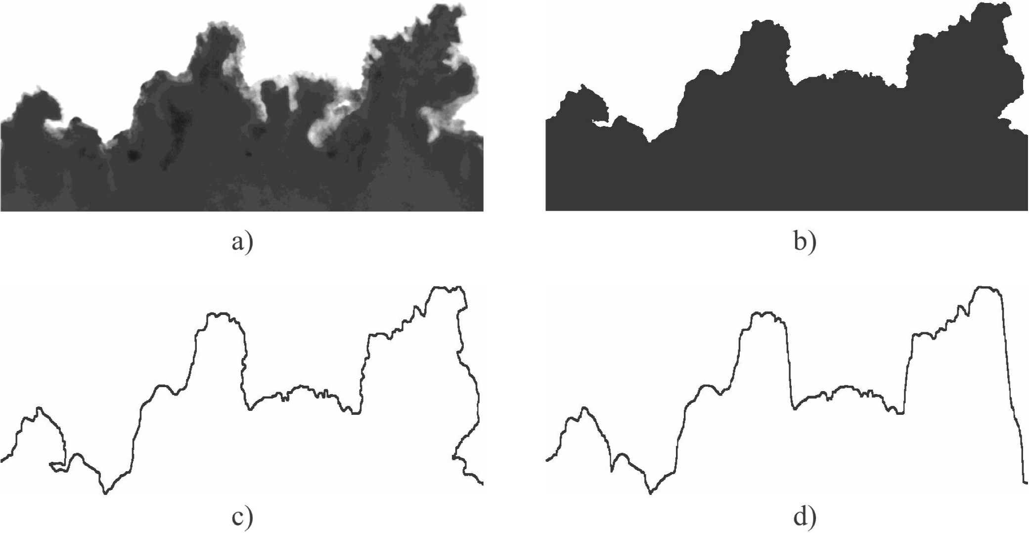
Figure 2. Transformation from self-avoiding walk to a single-valued series: a) Original image from a rough imbibition profile, b) Binary image of the rough imbibition profile, c) Self-avoiding profile, d) Self-avoiding profile transformed into a single-valued series.
Nevertheless, below we show that for the Koch curve20, which has a self-avoiding profile, this transformation leads to a significant error in the estimation of D. Therefore, there is a need to develop an efficient graphical method of fractal dimension estimation for self-avoiding profiles.
In what follows we propose a method of estimation of D for self-avoiding profiles called Fractionating estimator, and demonstrate its efficiency applying it to the classic examples of such curves: Koch curve, modified Koch curve21, G 2 Modified Koch curve22 and Weierstrass curve23.
3.1 Fractionating estimator (FE)
Using as reference the Hall-Wood estimator with scale
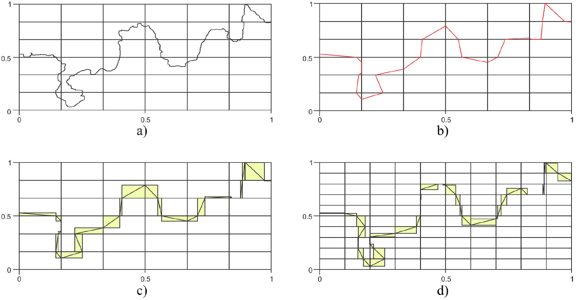
Figure 3. Operation of FE on a self-avoiding curve: a) grid (k = 6), b) adjusted broken line (k = 6), c) the box cover of the adjusted broken line (k = 6), d) the box cover of the adjusted broken line (k = 10).
Note that meanwhile the number of step k increases the broken line of FE approaches the interface curve. Furthermore, FE splits the rough self-avoiding curve not equidistantly, and in this way, it takes into account as much information from the rough curve both in rows and columns, “breaking it down" into fractional straight segments, preserving the Hall-Wood scale idea but counting boxes as in the Box-count estimator.
3.2 Fractal dimension estimation of Koch curve, modified Koch curves and Weierstrass curve
To verify the efficiency of FE, proposed above, a routine in Visual Basic for Applications for Corel Draw X3 was developed. The developed program was used for the estimation of fractal dimension by FE of the Koch curve (Fig. 4a) with theoretical D = 1.1609, single-value transformation of Koch curve (Fig. 4b), modified Koch curve (Fig. 4c) with theoretical D = 1.1609, G2 modified Koch curve (Fig. 4d) with theoretical D = 1.2924 and the Weierstrass curve (Fig. 4e) of the form:
for a = 0.5, b = 33 and theoretical D = 1.8017.
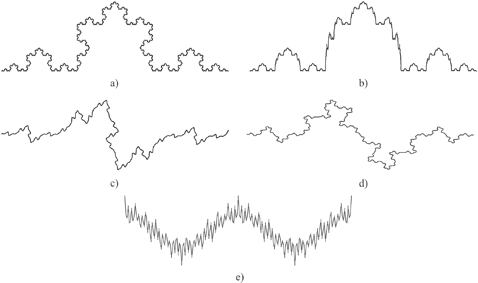
Figure 4. a) Koch curve generated with 4200 nodes, b) Single-valued transformation of Koch curve, c) modified Koch curve generated with 3200 nodes, d) G2 modified Koch curve generated with 6680 nodes, e) Weierstrass curve generated with 1571 nodes.
In addition the Box-count estimator included in software Benoit 1.31 and the plug-in for Image J software of FracLac 1.48, and the estimators Box-count, Hall-Wood, Variogram and Madogram of fractaldim package of software R, where used for the estimations of D for the considered fractals curves.
The FE routine was performed directly to the generated curve without transforming it to a single-valued profile, and the original vector graphic image was exported to .bmp format for Benoit 1.31 and FracLac 1.48, where the D was also estimated directly from the image using the Box-count estimator.
As the software R works only with numerical data the Koch curve was transformed into a single-valued curve (Fig. 4b) in .png format. After that the binarized image was interpreted as a matrix of ones and zeros, each column of ones are accounted to get a series of single-valued profile, from which D was estimated by Box-count, Hall-Wood, Variogram and Madogram estimators.
The results of the estimates of the single-valued Koch curve (Fig. 4b), are presented in a synthesized way by Boxplot graph in Fig. 5, where the theoretical and expected dimension D = 1.2619 of the Koch curve is marked with dotted horizontal line.
Numerical results of the average estimates for a single-valued profile generated from the Koch curve obtained using the fractaldim package are presented in Table I.
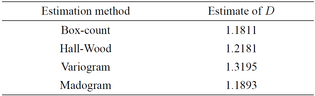
From Table I it can be seen that the Hall-Wood estimator has the best performance, followed by Variogram, but none of the considered estimators gives a reliable estimate. Above mentioned results confirm the fact that the transformation of the original Koch curve into a single-valued profile leads to a significant errors in fractal dimension estimation.
Now, performing the estimation of D for the original Koch curve by FE, t was observed, as expected, that for self-avoiding interfaces the basic proportionality of Hall-Wood method (3) does not hold (Fig. 6).

At the same time, from Fig. 7, one can observe a power law behavior with the coefficient of determination R2 very close to 1 and the estimated value of D obtained by the proposed FE method is 1.2609 and approximates the theoretical D = 1.2619.
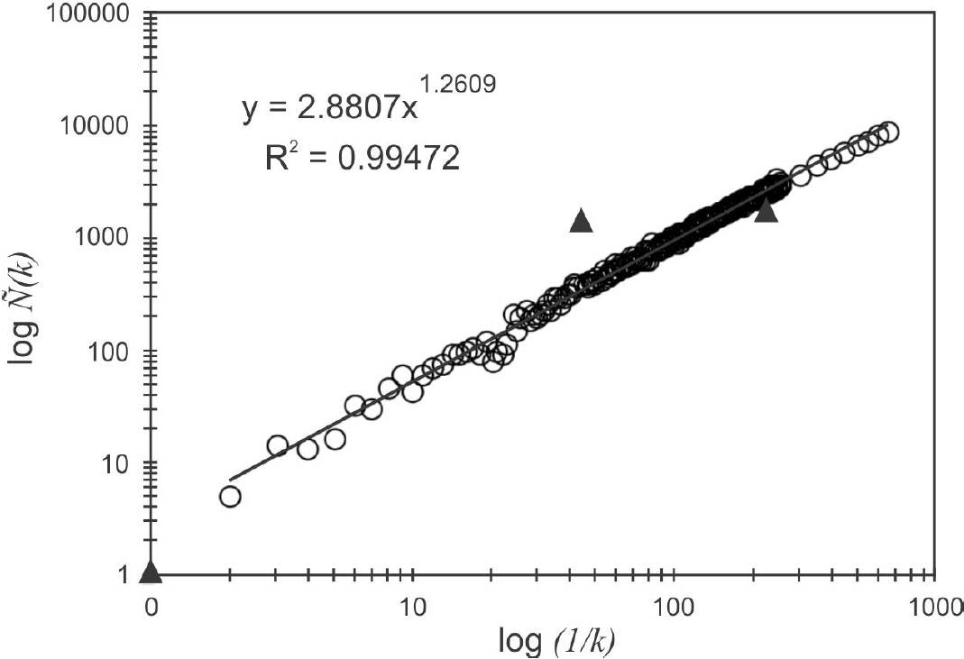
In Fig. 7 the points indicated as triangles correspond to outliers and were not taken into account for the linear regression fit, as the value of the coefficient of determination R2 in that case reduces to R2 = 0.9873. The fractal dimension of the original Koch curve was also estimated by the Box-count estimator using the software Benoit and FracLac. The same estimators were used for modified Koch curve (Fig. 4c), G2 modified Koch curve (Fig. 4d) and Weierstrass curve (Fig. 4e).
The values of estimates of fractal dimensions of the Koch curve, modified Koch curve, G2 modified Koch curve and Weierstrass curve obtained by FE, Benoit and FracLac methods are presented in Table II.
Table II. Fractal dimension estimates of theoreticall self-avoiding curves: Koch curve, modified Koch curve, G 2 modified Koch curve and Weirstrass curve.
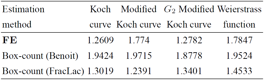
As it can be seen from Tables I and II, the developed FE method gives significantly better estimates for both curves studied as compared to the commonly used methods of estimation.
Furthermore, as the scaling behavior of a profile with overhangs (Fig. 2), can lead from self-affinity to multi-affinity by the removal of overhangs in the representation of real interface by single-valued profile24, the proposed method avoid this problem and there is no need of further study scaling and universality for a varied self-avoiding curves.
4. Conclusions
In this work a study of graphical and statistical estimators such as Box-count, Hall-Wood, Variogram, and Madogram for self-avoiding curves embedded in
A new method for the estimation of fractal dimension for self-avoiding rough interfaces based on the efficiency of Hall-Wood estimator was developed and evaluated. The estimates of fractal dimensions obtained by the proposed method of Fractionating Estimator for the considered fractal curves closely approximate the theoretical dimension of the fractals and give more precise estimations as compared with the commonly used estimators. Results obtained validate the application and use of the proposed method for the calculation of D for the rough interfaces as well as time series.

