


 text new page (beta)
 English (pdf)
 Article in xml format
 Article references
 Send this article by e-mail
 Cited by SciELO
  Similars in
SciELO
Similars in
SciELO 
 Permalink
1. Introduction
Nonclassicality is of fundamental importance in quantum physics. It is an essential ingredient in quantum-enhanced technologies. For instance, it is crucial for the generation of entanglement1-5. In phase-space representation, nonclassicality is closely related to the negativity of the Wigner function6. By means of the negative part of the Wigner function in the phase space, indicators are proposed by Benedict et al.7,8 and Kenfack et al.9 to measure the degree of the nonclassicality of a quantum state. They are used, for example, to characterize the nonclassicality in optomechanical systems10,11. Indeed, the negativity of the Wigner function is a also key resource in many fields of quantum physics, e.g., in quantum optics12 and in quantum computation13-16. It is proposed as a necessary resource of the quantum computation, which is closely related to the contextuality13-15. In addition, the negativity of the Wigner function is also of special interest in mechanical systems11,17-19.
During the past decade, mechanical systems are emerging as good candidates for studying the quantum mechanical behavior and the nonclassical states at the mesoscopic and even macroscopic scales17-24. In the fields related to mechanical systems, driven nonlinear systems are of fundamental and technical interests18,20-30. They are key ingredients in many fields such as optomechanical systems18-20, nanomechanical resonators17,24-27 and Josephson bifurcation amplifiers29,30. Generally, in driven nonlinear systems, the time evolution of the quantum state can be influenced by the external driving source. Due to the potential applications of the nonclassicality and the driven nonlinear system, it is necessary to explore the relations of the nonclassicality to the driving frequency in driven nonlinear systems during the time evolution of the quantum state. This is also the interest of this paper.
The investigations are performed with a Duffing-type oscillator, which is a typical driven nonlinear system. The nonclassicality is measured by the indicator which is defined based on the negativity of the Wigner function. When using the Gaussian state as the initial Wigner function, the time evolution of the nonclassicality of the quantum state has significant driving frequency dependence. For more detailed comparison, the time-average of the nonclassicality indicator is used to evaluate the frequency dependence of the time evolution of the nonclassicality. Its frequency response curve has a pronounced peak, near which the nonclassicality of the state is enhanced during the time evolution. This can be attributed to the influence of the external driving source on the energy levels involved in the time evolution of the Wigner function and can be understood by means of the Floquet theories. Furthermore, for different centers of the initial Wigner function, good correspondences are observed between the frequency response curves of the time-average of the nonclassicality indicator and those of the classical mean square amplitude. This arises from the relation of the classical mean square amplitude to the energy levels involved in the evolution of the system. Similarly, the time evolution of the nonclassicality indicator also has remarkable frequency response with a superposition of the coherent states as the initial Wigner function. Meanwhile, correspondences can be seen between the frequency response curves of the nonclassicality indicator and those of the classical mean square amplitude, although superpositions of coherent states are usually regarded as typical nonclassical states.
The remainder of the paper is structured as follows. In Sec. 2, the nonclassicality indicator and the Duffing-type system used here are presented. In Sec. 3, the frequency response of the nonclassicality indicator during the quantum evolution is investigated with the Gaussian state as the initial Wigner function, after which its relation to the frequency response of the underlying classical dynamics is analyzed. Section 4 is dedicated to investigate the frequency response of the nonclassicality with a superposition of two coherent states as the initial Wigner function. Besides, Sec. 5 is devoted to the conclusions.
2. Nonclassicality indicator and the Duffing-type system
As mentioned above, the negativity of the Wigner function has potential application in quantum realm. It is usually regarded as a good indication of a quantum state’s nonclassical character6-9. The nonclassicality indicator used here is defined by Kenfack et al.9 by means of the negativity of the Wigner function. It reads
which equals to the doubled volume of the integrated negative part of the Wigner function in the phase space. It equals to zero for coherent states, whose Wigner functions are non-negative. A similar indicator is proposed by Benedict et al.7,8 based on the negative volume of the Wigner function. It can be written as ν=δ/(δ+1) with 0≤𝜈<1. Apart from the negativity of the Wigner function, nonclassicality can also be measured by, for example, the photon number31, the interference in the phase space32 and the Tsallis entropy33. The latter two have similar behavior to the nonclassicality indicator 𝛿 for Wigner functions32,33.
The system used here is a Duffing-type oscillator. Its Hamiltonian can be written as
with
where 𝜅 gives the strength of the nonlinearity and 𝑆𝑞cos𝜔𝑡 stands for the external driving source. It is of both theoretical and experimental interests and is also often used in the studies related to optomechanical and nanomechanical devices25-29.
The state 𝛹(𝑡) of the system at the time 𝑡 is described by the Wigner function
 (4)
(4)
As a typical phase-space distribution function, the Wigner function provides a convenient framework to test the quantum-classical correspondence and offers a way for quantum state reconstruction via quantum tomography34,35. The Wigner function and its negativity can also be measured experimentally, for example, in quantum optics36,37. The time evolution of the Wigner function follows from the Schrödinger equation
where the arrows indicate in which direction the derivatives act and the sin function can be expanded in a power expansion in ℏ. In the classical limit, Eq. (5) corresponds to the classical Liouville equation.
Following Eqs. (1) to (5), the time evolution of the nonclassicality of the system (2) and its relations to the driving frequency are numerically investigated. For the sake of simplicity, atomic units are used in the following sections with 𝑚=ℏ= 𝜔 0 =1.
3. Gaussian Wigner function
3.1 Frequency response of the nonclassicality during the quantum evolution
Gaussian states, also known as coherent states, are widely used in the theoretical and experimental works. They are considered as being closest to the corresponding classical states, providing a way to compare the classical and quantum dynamics38. In the Wigner representation, a Gaussian state can be written as
with ( 𝑞 0 , 𝑝 0 ) as its center. Its value of the nonclassicality indicator 𝛿=0. This is consistent with the above descriptions of coherent states. However, the value of 𝛿 will no longer be equal to zero during the quantum evolution of a driven anharmonic oscillator like (2). Furthermore, its value evolution can be influenced by the driving frequency during the quantum evolution. These will be illustrated and discussed later.
With the Gaussian state (6) as the initial Wigner function, we numerically investigate the value of the nonclassicality indicator 𝛿 during the time evolution of the Wigner function in the Duffing-type system (2). The parameter values are 𝜅=0.1 and 𝑆=1. Without loss of generality, we consider here the case of a stiffening nonlinearity with 𝜅>0. Both values of 𝜅 and 𝑆 can influence the evolution of the Wigner function. However, they are taken to be constants in order to focus on the driving frequency dependence of the nonclassicality.
It is found from the numerical results that the value of the nonclassicality indicator, which is initially equal to zero, evolves with the time. Moreover, the time evolution of the nonclassicality indicator significantly depends on the frequency of the driving source. This can be observed in the main figure of Fig. 1. In the main figure of Fig. 1, we present three typical plots of the time evolution of the nonclassicality indicator for ( 𝑞 0 , 𝑝 0 )=(−1.5,0). From bottom to top, they correspond to 𝜔=0 (black solid line), 𝜔=3 (blue dotted line) and 𝜔=1.5 (red dashed line). As can be seen the main figure of Fig. 1, the increase of ?? in the beginning is faster for 𝜔=1.5 than those for 𝜔=0 and 𝜔=3.
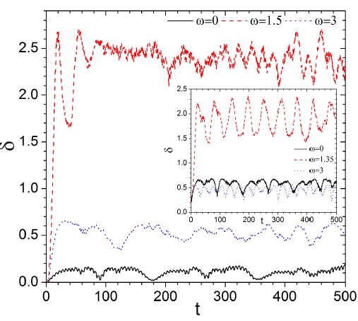
Figure 1 Nonclassicality indicator ± versus the time t with a Gaussian wave packet as the initial Wigner function. The center of the initial Wigner function is (q0; p0) = (¡1:5; 0). The values of the driving frequencies are 0 (black solid line), 1:5 (red dashed line) and 3 (blue dotted line). Inset: the same as in the main figure but with a superposition of two coherent states as the initialWigner function, whose centers (§q0; p0) are (§1:5; 0). The values of the driving frequencies in the inset figure are 0 (black solid line), 1:35 (red dashed line) and 3 (blue dotted line).
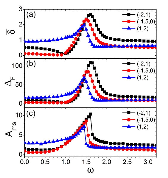
Figure 2 Frequency response curves of (a) the time-average of the nonclassicality indicator ±, (b) the time-average of the dispersion of the Wigner function in the Fourier domain ¢F and (c) the classical mean square amplitude Ams. In each panel, the four curves are obtained with (q0; p0) equal to (¡2; 1) (black squares), (¡1:5; 0) (red circles) and (1; 2) (blue triangles). The increments of ! are 0:05 for the interval [1; 2] and 0:1 for the other intervals.
Moreover, after the initial increase the value of 𝛿 is much larger for 𝜔=1.5 than those for 𝜔=0 and 𝜔=3, though it oscillates with time.
For more detailed comparison, further numerical investigations are made with the driving frequency increasing from 0 to 3. The results for the nonclassicality indicator 𝛿 are presented in Fig. 2(a). As can be found from Fig. 1, the value of 𝛿 oscillates around some mean value after the increase at the beginning. Therefore, in Fig. 2(a), the frequency dependence of the nonclassicality indicator is characterized by its average over the time, i.e. 𝛿 = 𝜏 −1 0 𝜏 𝛿(𝑡)𝑑𝑡 with 𝜏=500. The results for ( 𝑞 0 , 𝑝 0 )=(−1.5,0) are marked by red circles in Fig. 2(a). In Fig. 2(a), the value of 𝛿 for ( 𝑞 0 , 𝑝 0 )=(−1.5,0) varies significantly with the driving frequency 𝜔 and reach its maximum when 𝜔=1.5. Especially, its frequency response curve has a pronounced response peak, near which the nonclassicality is enhanced. For further confirmation, calculations are performed with ( 𝑞 0 , 𝑝 0 )=(−2,1) and ( 𝑞 0 , 𝑝 0 )=(1,2). The frequency response curves of 𝛿 for ( 𝑞 0 , 𝑝 0 )=(−2,1) and ( 𝑞 0 , 𝑝 0 )=(1,2) are also presented in Fig. 2(a). They are marked with black squares and blue triangles. As displayed by Fig. 2(a), all the frequency response curves of 𝛿 for different ( 𝑞 0 , 𝑝 0 ) have notable response peaks, although the positions and amplitudes of their peaks are different from each other.
As shown by the definition of 𝛿, the increase of the nonclassical indicator 𝛿 arises from the enhancement of the negativity of the Wigner function in the phase space. The latter can be directly seen from the snapshot of the Wigner function during the quantum evolution. As illustrative examples, typical snapshots of the Wigner functions at 𝑡=200 are presented in Fig. 3. They are obtained with ( 𝑞 0 , 𝑝 0 )=(−1.5,0) and correspond to the three curves in Fig. 1. Their driving frequencies from (a) to (c) equal to 𝜔=0, 𝜔=1.5 and 𝜔=3 (𝜔=1.5 corresponds to the peak value of the frequency response curve of 𝛿 for ( 𝑞 0 , 𝑝 0 )=(−1.5,0) in Fig. 2(a)). From Fig. 3, one can observe the variance of the negativity of the Wigner function with the driving frequency. Especially, the Wigner function at 𝑡=200 has much larger negative part for 𝜔=1.5 than for 𝜔=0 and 𝜔=3. Besides, it also has more components and more fringes for 𝜔=1.5 than those for 𝜔=0 and 𝜔=3. Indeed, as a result of the quantum interference, the fringes of the Wigner function are closely related to the negativity of the Wigner function. The latter has been used to describe the interference effects in the quantum domain34,39 and can also be regarded as an indicator of the nonclassicality32.
3.2 Influences of the driving frequency on the evolution of the nonclassicality
As shown above, the increases of the nonclassicality and negativity of the Wigner function are closely related to the fringes of the Wigner function in the phase space. It is known that the fringes of the Wigner function arise from the interference between the energy levels involved in the quantum evolution. The latter can be influenced by the driving source and such influence is dependent on the driving frequency. This can be understood from the Floquet theory.
According to the Floquet theory40,41, for a system like (2), the quantum state |𝛹(𝑡)⟩ at the time 𝑡 can be expressed as
where the coefficients $ {\gamma _\alpha } = \left\langle {{{\varphi _\alpha }(0)}} \mathrel{\left | {\vphantom {{{\Phi _\alpha }(0)} {\Psi (0)}}} \right. \kern-\nulldelimiterspace} {{\Psi ( 0)}} \right\rangle$. {| 𝜑 𝛼 (𝑡)⟩} are the Floquet eigenstates of the system ([Eq:DuffH]) with { 𝜀 𝛼 } as their corresponding Floquet energies, satisfying
Both | 𝜑 𝛼 (𝑡)⟩ and 𝜀 𝛼 are dependent on the driving fequency . In addition, | 𝜑 𝛼 (𝑡)⟩ are periodic in time and obey | 𝜑 𝛼 (𝑡+𝑇)⟩=| 𝜑 𝛼 (𝑡)⟩ with 𝑇=2𝜋/𝜔. They can be expanded in a Fourier series, i.e.
where
In this view, 𝜑 𝛼 (𝑡) can be regarded as a superposition of stationary states with energies equal to 𝜀 𝛼,𝑘 = 𝜀 𝛼 −𝑘𝜔ℏ.
By means of the eigenbasis of the undriven Hamiltonian 𝐻 0 , the Floquet eigenstates of the driven system can be rewritten as
where 𝜓 𝑛 satisfy 𝐻 0 𝜓 𝑛 = 𝐸 𝑛 𝜓 𝑛 and 𝑐 𝛼,𝑘,𝑛 =⟨ 𝜓 𝑛 | 𝐶 𝛼,𝑘 ⟩ are time independent. Accordingly, the density operator 𝛹(𝑡) 𝛹(𝑡) can be expressed as
Its Wigner transform is
Where
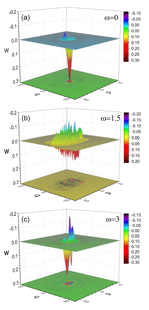
Figure 3 Plots of the Wigner function W(q; p; t) at the time t = 200 for (a) ! = 0, (b) ! = 1:5 and (c) ! = 3 with (q0; p0) = (¡1:5; 0). The values of the Wigner function are plotted in reverse scale for the sake of comparing the negative part of the Wigner functions.
As can be seen from Eq. (13), the time evolution of the Wigner function of the system can be regarded as a combination of a set of components. These components are related to the Floquet energy levels of the driven system (for simplicity, we shall use the term “energy levels” as “Floquet energy levels”) and evolve like small packets, whose periods depend on ( 𝜀 𝛼,𝑘 − 𝜀 𝛽,𝑘′ )/ℏ (similar conclusions can be found in Refs.42-45).
As a coherent state closest to the corresponding classical state, the Wigner function of the system 𝑊(𝑥,𝑝;𝑡) at 𝑡=0 is a smoothed Gaussian wave packet. The value of its nonclassicality indicator 𝛿=0. However, the components of the Wigner function with respect to different energy levels evolve with different periods for a driven nonlinear system like (2), as displayed in Eq. (13). They depart from and interfere with each other during the quantum evolution. This results in the emergence and evolution of the interference fringes of the Wigner function, and thus leads to the increase and evolution of the nonclassicality indicator. In addition, as can be observed in the main figure of Fig. 1, the nonclassicality indicator oscillates around some mean value for the same driving frequency after the growth at the beginning. This is because the quantum motion is quasi-periodic, since any component in the Wigner function (13) resumes its original form after some period of time. However, its periodicity can be deceased as the number of the energy levels involved in the time evolution of the Wigner function increases.
The energy levels involved in the quantum evolution can be influenced by the external driving source and are dependent on the driving frequency40,41. This induces the driving frequency dependence of the time evolution of the nonclassicality indicator and can be seen by means of the Floquet equation ([Eq:FloqSch]). In terms of 𝐶 𝛼,𝑘 and | 𝜓 𝑛 ⟩, Eq. (8) reads
where 𝑄 𝑛,𝑛′ = 𝜓 𝑛 𝑞 𝜓 𝑛′ (similar results can be found in Refs.41,46). Multiplying with 𝑒 −𝑖𝑙𝜔𝑡 and taking the time average over one period of the driving, it becomes
As can be seen from Eq. (16), only Floquet eigenstates with the corresponding eigenvalues 𝜀 𝛼,𝑙 close to 𝐸 𝑛 will be efficiently coupled. In other words, the energy-level transitions can be enhanced, as 𝜀 𝛼,𝑙 → 𝐸 𝑛 (i.e., 𝜀 𝛼,𝑙 − 𝐸 𝑛 →0). This is similar to what happens in a classical driven system near the region of the resonance.
Enhancement of the energy-level transitions results in more energy levels involved in the time evolution of the Wigner function. In this case, the time evolution of the Wigner function involves more components, which are related to different energy levels. This can be seen from Fig. 3. In Fig. 3, the Wigner function at 𝑡=200 has broken into small components. Especially, the Wigner function has much more small components for the peak frequency 𝜔=1.5 than for 𝜔=0 and 𝜔=3. This means the energy levels involved in the quantum evolution are greatly increased near the peak frequency 𝜔=1.5. As mentioned above, the increase of the energy levels involved in the quantum evolution can decrease the periodicity of the time evolution of the Wigner function. This is consistent with the main figure of Fig. 1. In the main figure of Fig. 1, the periodicity of the time evolution of the nonclassicality indicator for 𝜔=1.5 is much less obvious than those for 𝜔=0 and 𝜔=3.
Furthermore, due to the interference between different energy levels, the increase of the energy levels involved in the quantum evolution is accompanied with the increase of the fringes of the Wigner function. The latter corresponds to the increase of the negativity of the Wigner function and thus to the enhancement of the nonclassicality32,47. This can also be confirmed by Fig. 3. In Fig. 3, the Wigner function has more interference fringes and larger negative volume for 𝜔=1.5 than for 𝜔=0 and 𝜔=3.
Indeed, the Wigner function discussed here can be regarded as a two dimensional gray-scale image. According to the image-processing theories, the fringes of the Wigner function in the phase space (or the oscillations of the Wigner function in the phase space) can be investigated by the Fourier transform48. The increase of the interference fringes of the Wigner function in the phase space corresponds to the increase of the dispersion of the Wigner function in the Fourier domain. Thus, the dispersion of the Wigner function in the Fourier domain can be used as an indicator of the interference fringes of the Wigner function in the phase space. It can be evaluated by the variance of the Wigner function in the Fourier domain 𝛥 𝐹 = 𝛥𝑞 𝐹 𝛥𝑝 𝐹 , where 𝛥𝑞 𝐹 and 𝛥𝑝 𝐹 are the variances along the 𝑞 𝐹 and 𝑝 𝐹 directions respectively ( 𝑞 𝐹 and 𝑝 𝐹 are the space frequencies correspond to 𝑞 and 𝑝). Similar to 𝛿 , the time-average of 𝛥 𝐹 (i.e. 𝛥 𝐹 ) is used to compare the degree of the oscillations of the Wigner function in the phase space during the time evolution for different driving frequencies. The frequency response curves of 𝛥 𝐹 for different ( 𝑞 0 , 𝑝 0 ) are illustrated in Fig. 2(b). They have good correspondences to the frequency response curves for the nonclassicality indicator in Fig. 2(a). This confirms the above conclusion that the driving source influences the nonclassicality via influencing the energy levels involved in the quantum evolution and the interference fringes of the Wigner function.
3.3 Correspondence between the frequency responses of the nonclassicality and the classical dynamics
As discussion above, the driving source influences the nonclassicality of the quantum state via influencing the energy levels involved in the quantum evolution. Moreover, in the further investigations, a good correspondence is found between frequency response curve of the nonclassicality indicator and that of the classical mean square amplitude.
The classical mean square amplitude reads
where 𝑞(𝑡) is obtained by classical Hamilton’s equations with ( 𝑞 0 , 𝑝 0 ) as the initial condition. It is also an average over the time scale.
The frequency response curves of 𝐴 𝑚𝑠 for different ( 𝑞 0 , 𝑝 0 ) are presented in Fig. 2(c). They are obtained with ( 𝑞 0 , 𝑝 0 ) equal to (−2,1) (black squares), (−1.5,0) (red circles) and (1,2) (blue triangles). Comparing Figs. 2(a) and 3(c), clear correspondences can be seen between the frequency response curves for the nonclassicality indicator and those for the classical mean square amplitude. Specifically, the response peak of 𝛿 in Fig. 2(a) and that of 𝐴 𝑚𝑠 in Fig. 2(c) for the same ( 𝑞 0 , 𝑝 0 ) reach their maximum near the same driving frequency. They are similar to each other in amplitude, position and shape. Meanwhile, the frequency response curves in Figs. 2(a) and 2(c) for different ( 𝑞 0 , 𝑝 0 ) are also similar to each other in the relative position and height. These suggest the connections between the frequency response of the time evolution of the nonclassicality and that of the mean square amplitude of the underlying classical dynamics.
Following the Parseval’s theorem , for a large 𝜏,
where
is the power spectral density of the classical trajectory and 𝜂 denotes the angular frequency. According to the classical-quantum theories50-52, 𝐼(𝜂) is closely related to the quantum mechanical spectrum with the angular frequencies 𝜂 corresponding to the energy-level transitions. Thus, the integral of 𝐼(𝜂) with respect to 𝜂 can be used as an indicator for the energy levels involved in the evolution of the system. As discussion above, the energy levels involved in the evolution of the system are responsible for the emergence of the interference fringes of the Wigner function. Accordingly, the variation of 𝐴 𝑚𝑠 with the driving frequency 𝜔 can reveal the driving frequency dependence of the interference fringes of the Wigner function during the quantum evolution. This can be confirmed by the correspondence between the frequency response curves of 𝛥 𝐹 in Fig. 2(b) and those of 𝐴 𝑚𝑠 in Fig. 2(c). The increase of the interference fringes of the Wigner function can enhance the nonclassicality of the Wigner function, as shown in the previous section. Thus, correspondences can also be found between the frequency response curves of the time-average of the nonclassicality indicator 𝛿 and those of classical mean square amplitude 𝐴 𝑚𝑠 , as shown by Figs. 2(a) and 2(c).
4. Superposition of two coherent states
In the Sec. 2, the time evolution of the nonclassicality indicator shows significant dependence on the driving frequency when using Gaussian coherent states as the initial Wigner functions. This arises from the influence of the driving source on the energy levels involved in the quantum evolution. In this view, the frequency dependence of the nonclassicality indicator during the time evolution should hold true to some extent by taking a superposition of two coherent states as the initial Wigner function. The latter is constructed by choosing two coherent states 𝜙 ± localized in two distant points of the configuration space (± 𝑞 0 , 𝑝 0 ) . Its wave function reads
where 𝜙 ± (𝑞)= 𝜋 −1/4 exp[− (𝑞± 𝑞 0 ) 2 /2+𝑖 𝑝 0 (𝑞± 𝑞 0 )] and 𝑁 is the normalization constant satisfying 𝑁=[1+cos(2 𝑞 0 𝑝 0 )exp(− 𝑞 0 2 ) ] −1/2 9,32,33. The Wigner function of the wave function (20) can be written as
where
And
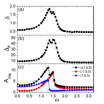
Figure 4 Frequency response curves of (a) the time-average of the nonclassicality indicator ± and (b) the time-average of the dispersion of the Wigner function in the Fourier domain ¢F with a superposition of two coherent states as the initial Wigner function. The two peaks centers of the initial state (§q0; p0) for (a) and (b) are (§1:5; 0). In (c), the curves marked by red circles and blue triangles denote the frequency response curves of the classical mean square amplitude Ams for (q0; p0) = (¡1:5; 0) and (q0; p0) = (1:5; 0) respectively, and their superposition (or sum) is marked by black squares.
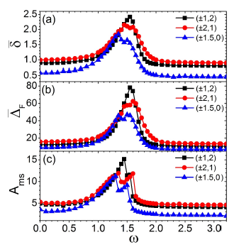
Figure 5 Frequency response curves of (a) the time-average of the nonclassicality indicator ± and (b) the time-average of the dispersion of the Wigner function in the Fourier domain ¢F for different initial Wigner functions. Each initial Wigner function is a superposition of two coherent states. In (a) and (b), the peak centers of the initial Wigner functions (§q0; p0) are (§1; 2) (black squares), (§2; 1) (red circles) and (§1:5; 0) (blue triangles). In (c), the curve for (§q0; p0) denote the superposition of the two frequency response curves of the classical mean square amplitude Ams for (q0; p0) and (¡q0; p0) with (q0; p0) equal to (1; 2) (black squares), (2; 1) (red circles) and (1:5; 0) (blue triangles).
As further investigation and confirmation, the state (21) is taken as the initial Wigner function of the system in this section. The values of 𝜅 and 𝑆 are the same as those in the previous sections. The curves of the nonclassicality indicator 𝛿 versus the time 𝑡 are displayed in the inset figure of Fig. 1. They are obtained with (±1.5,0) as the centers of the two coherent states (± 𝑞 0 , 𝑝 0 ). Their values of the driving frequencies are 0 (black solid line), 1.35 (red dashed line) and 3 (blue dotted line). From the inset figure of Fig. 1, it can be seen that the time evolution of the nonclassicality indicator 𝛿 is significantly dependent on the driving frequency, when using a superposition of two coherent states as the initial Wigner function. This is the same to the case of the Gaussian state in the previous section.
Similarly, the time-averages of 𝛿 are calculated with 𝜔 increasing from 0 to 3. Their frequency response curves are displayed in Fig. 4(a) (𝜏=500). In Fig. 4(a), the frequency response curve of 𝛿 have a remarkable response peak, which occurs near 𝜔=1.35. As discussion in the previous section, this arises from the influence of the driving source on the energy levels involved in the quantum evolution, and can be confirmed by the frequency response curve of 𝛥 𝐹 . The frequency response curve of 𝛥 𝐹 is displayed in Fig. 4(b). It is obtained under the same conditions as in Fig. 4(a). Comparison of Figs. 4(a) and 4(b) indicates a correspondence between the frequency response curves of 𝛿 and 𝛥 𝐹 in curve shape and peak position. This reveals the growth of the fringes of the Wigner function and the increase of the energy levels near the peak of the frequency response of 𝛿 .
Furthermore, the Wigner function of the state (21) is a superposition of two Gaussian coherent states. In this view, the correspondence between the frequency response of the nonclassicality and that of the classical dynamics for the Gaussian coherent state could emerge to some extent in the evolution of the Wigner function with the state (21) as the initial Wigner function. This can be seen by comparing Figs. 4(a) and 4(c).
In Fig. 4(c), the curves marked by red circles and blue diamonds denote the frequency responses of the classical mean square amplitude 𝐴 𝑚𝑠 for ( 𝑞 0 , 𝑝 0 )=(−1.5,0) and ( 𝑞 0 , 𝑝 0 )=(1.5,0) respectively. By comparing Figs. 4(a) and 4(c), one can see that the peak of the frequency response curve of 𝛿 occurs in the frequency interval where the peaks of the frequency response curves of 𝐴 𝑚𝑠 for ( 𝑞 0 , 𝑝 0 )=(−1.5,0) and ( 𝑞 0 , 𝑝 0 )=(1.5,0) appear. This can be viewed as some kind of resonance and can be confirmed by the superposition (or summation) of the two frequency response curves of 𝐴 𝑚𝑠 for ( 𝑞 0 , 𝑝 0 )=(−1.5,0) and ( 𝑞 0 , 𝑝 0 )=(1.5,0). The superposition of the two frequency response curves of 𝐴 𝑚𝑠 for ( 𝑞 0 , 𝑝 0 )=(−1.5,0) and ( 𝑞 0 , 𝑝 0 )=(1.5,0) is marked by black squares in Fig. 4(c). It varies with the driving frequency in a similar manner to the frequency response curve of 𝛥 𝐹 in Fig. 4(b) and has a correspondence to the frequency response curve of 𝛿 in Fig. 4(a).
For further comparison, numerical calculations are performed with (±1,2) and (±2,1) as the peak centers (± 𝑞 0 , 𝑝 0 ). The frequency response curves of 𝛿 for the peak centers (±1,2) (black squares), (±2,1) (red circles) and (±1.5,0) (blue triangles) are all presented in Fig. 5(a). All of them have remarkable response peaks and have clear correspondences to the frequency response curves of 𝛥 𝐹 in Fig. 5(b). Besides, in Fig. 5(c), we presents the superposition of the two frequency response curves of the classical mean square amplitude for ( 𝑞 0 , 𝑝 0 )=(±1,2) (black squares), ( 𝑞 0 , 𝑝 0 )=(±2,1) (red circles) and ( 𝑞 0 , 𝑝 0 )=(±1.5,0) (blue triangles). Correspondences can be found between the frequency response curves in Figs. 5(a), 5(b) and 5(c) for different (± 𝑞 0 , 𝑝 0 ) in peak position and peak amplitude. This confirms the above conclusions that the driving frequency influences the interference fringes and nonclassicality of the Wigner function via influencing the participation of the energy levels in the quantum evolution.
5. Conclusions and Discussions
The frequency response of the nonclassicality is investigated in a driven nonlinear system by using the Gaussian state and the superposition of two coherent states as the initial Wigner functions. For different initial Wigner functions, the frequency response of the nonclassicality during the quantum evolution has significant response peak, near which the nonclassicality and the negativity of the Wigner function are greatly increased. This can be used for example to enhance the nonclassicality of the quantum state in driven nonlinear systems. The latter is a key resource in quantum-enhanced technologies. Moreover, the frequency response of the nonclassicality during the quantum evolution has a good correspondence to the frequency response curve of the classical mean square amplitude. This is because the classical mean square amplitude reveals the energy-level transitions. In other words, the frequency response of the classical mean square amplitude can be regarded as an indicator of the frequency response of the energy-level transitions in the classical regime. The energy-level transitions involved in the quantum evolution are responsible for the increase of the interference fringes of the Wigner function as well as the increase of the nonclassicality indicator, as discussed in Sec. 3B. Accordingly, correspondence emerges between the frequency responses of the nonclassicality indicator and the classical mean square amplitude.
The conclusions are obtained here with a model of the Duffing-type oscillator. However, they should hold true to some extant for other driven nonlinear systems, due to the relations of the energy-level transitions to the classical mean square amplitude. In this view, the frequency response of the classical mean amplitude suggests a simple way to indicate the driving frequency dependence of the nonclassicality in driven nonlinear systems, since it is easy to be calculated. Its response peak can be used to predict the frequency interval where the nonclassicality can be greatly enhanced by the external driving source. Besides, the frequency response of the nonclassicality is investigated here by means of the negativity of the Wigner function. As mentioned above, the negativity of the Wigner function has attracted particular attentions due to its potential applications in quantum optics and quantum computations. Thus, the investigations presented here may shed some light on the applications of the negativity of the Wigner function.

