1. Introduction

Multiparticle¹ Collision Dynamics (MPC) is a simulation technique introduced by Malevanets and Kapral^2,3, that can be used to simulate the physical behavior of a simple fluid at the mesoscopic scale. In comparison with similar methods like Brownian Dynamics , Stokesian Dynamics^4,5 or the Lattice Boltzmann technique^7-9, MPC possesses special features that make it more appealing for the simulation of complex systems. For instance, since MPC is based on particles, it can be easily coupled to polymers or colloids^10-13, a task that is hard to achieve by methods based on grids like Lattice Boltzmann. In addition, MPC captures the hydrodynamic behavior of the fluid around the embedded particles and, thus, it naturally incorporates hydrodynamic interactions¹⁰, which are absent in Brownian Dynamics and must be given through an analytical representation of the mobility tensor in Stokesian Dynamics. Furthermore, the MPC algorithm is stochastic and gives rise to hydrodynamic fluctuations and Brownian forces on the suspended particles^10,14-18. Finally, the MPC algorithm is relatively simple and has been analytically studied from kinetic and projection operator theories^19-22, finding an excellent agreement with the simulation results. This has confirmed that a very good understanding of the method has been achieved and, in turn, has given confidence in using MPC for simulating physical systems as diverse as suspensions of polymers²³ and colloids^3,10, polymers under flow^15.24,25, flow around objects^26,27, vesicles under flow²⁸.

In the simplest case, MPC simulations are carried out by implementing the so-called periodic boundary conditions, which imply that the simulated fluid is a portion of a much larger, actually infinite, system. However, for some applications of diffusion in confined systems^29,30, some of which are relevant for microfluidic and biological problems^28,31, it could be convenient to simulate flow of spatially constrained MPC fluids. One option for extending the basic MPC algorithm to include the presence of spatial constrains, is to implement hard walls which are usually incorporated as surfaces that elastically reflect back those particles coming from the fluid phase. Although this extension requires additional considerations to obtain the correct behavior of the fluid at the confining boundary, it has been used successfully to reproduce hydrodynamic flows in diverse situations^2,28,32-35. In two recent publications^1,36, we have introduced another option for simulating the flow of spatially constrained MPC fluids in which confinement is achieved by considering explicit forces on the particles of the fluid phase that are exerted by surfaces that represent physical walls. Although this method is more expensive than the hard wall technique from the point of view of computations, it has the advantage of yielding simulations that are closer to an actual physical situation, as long as fluid-solid interactions are always mediated by explicit forces. We have used this method to simulate cylindrical¹ and plane Poiseuille flows³⁶.

In the present work, we shall show that this method can be used to simulate the behavior of a fluid in a more complex situation, namely, that corresponding to confinement between two coaxial cylinders. We will consider two specific scenarios in which an MPC fluid is forced to move through the space between the cylinders, first, by a uniform pressure gradient that points along the axial direction and, second, by a force field with azimuthal component only. In the former case, the method reproduces very well the flow expected from hydrodynamics. We will show that the numerical parameters that control the flow at the boundaries, presented previously in Ref. 1, can be directly used here to achieve flow with no-slip boundary conditions. In the latter case, we will notice that, since MPC fluids are compressible, a difficulty in applying the simulation technique appears consisting in the development of flows with non-uniform average densities. Therefore, simulations will be restricted to the case of small external centrifugal forces. In addition, the set of parameters used for controlling boundary conditions will be modified, since flow will be no longer axial but azimuthal. A series of experiments will be performed to determine this new set of parameters empirically. We will show that, under such conditions, our methodology allows for simulating the hydrodynamic flow between the cylinders expected for an incompressible fluid with no-slip boundary conditions, with a very satisfactory accuracy.

This paper is organized as follows. In Sec. 2, we will present the system to be simulated, as well as the MPC algorithm used to reproduce flow between coaxial cylinders. In particular, we will describe how the fluid-solid forces derived in Ref. 1 are applied in this situation. In Sec. 3, we will describe the results obtained for axial flow, while in Sec. 4 we will present the results for simulation of azimuthal flow. Finally, in Sec. 5 we will state our conclusions, and summarize the advantages and limitations of our approach.

2. MPC algorithm for confinement between coaxial cylinders

The physical system to be considered in the present work is schematically illustrated in Fig. 1. There, we define two coaxial cylindrical surfaces whose axes coincide with the z−axis of a Cartesian coordinate system. The radius of the external cylinder will be represented by ℛ 2 , while the internal radius will be denoted as ℛ 1 . Along the 𝑧 direction the system is assumed to have an extension 𝐿 𝑧 . From the point of view of the numerical method, it will be convenient to give these parameters characterizing the size of the system as multiples of a unit of length 𝑎. Thus in the following we can consider that ℛ 1 = 𝑛 1 𝑎, ℛ 2 = 𝑛 2 𝑎 and 𝐿 𝑧 = 𝑛 𝑧 𝑎, where 𝑛 1 , 𝑛 2 , and 𝑛 𝑧 are integers.

In MPC simulations a fluid is assumed to consist of 𝑁 point particles of mass 𝑚. These particles are represented as small black spheres in Fig. 1. The positions and velocities of the MPC particles will be represented by the vectors 𝑅 𝑖 and 𝑣 𝑖 , respectively, for 𝑖=1,2,…,𝑁. The fluid will be restricted to move in this geometry, by assuming that the internal and external cylinders are physical walls that interact with the MPC particles through repulsive potentials. Specifically, the interaction potential associated with the external wall, for an MPC particle located at 𝑅 𝑖 , will be written in the form

which was derived first in Ref. 1. In this expression, 𝜖 𝑆 denotes the strength of the fluid-solid interaction per unit area ; 𝜎 is the effective diameter of the interaction, with 𝜎 = 2 (1/6𝑛) 𝜎; and 𝑅 ∗ = 𝑅 ∗ ( 𝑅 𝑖 ) represents the closest point of the external wall to the position 𝑅 𝑖 . For the interaction with the internal wall, a completely analogous expression can be applied to obtain the corresponding potential 𝛷 int ( 𝑅 𝑖 ). The force on the particle due to its interaction with the walls, 𝐹 𝑖 wall , can be calculated from 𝐹 𝑖 wall =− 𝛻 ( 𝛷 ext + 𝛷 int ), although in practice, the radial separation between the internal and external walls is typically much larger than the interaction distances, in such a way that fluid particles do not interact simultaneously with both walls.

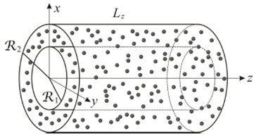
Figure 1 Schematic illustration of an ensemble of MPC particles (small black spheres) confined in the space between two coaxial cylinders. Quantities R1, R2, and Lz define the spatial extension of the system. 

As it has been shown in Ref. 1, with the purpose of simulating rough confining walls, it is convenient to apply the forces 𝐹 𝑖 wall in the anti parallel direction to the velocity with which the particles penetrate into the walls. In this scheme, particles that come into the region of interaction with the confining surfaces face different repulsing barriers. The procedure that can be implemented to determine the direction and magnitude of the forces caused by the external wall, was described in detail in Ref. 1, and can be straightforwardly extended to consider the interaction with the internal cylinder as well.

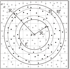
Figure 2 Schematic illustration of the procedure used to introduce virtual particles. The system is extended to a square region of size 2R2 + a in the xy-plane. The region between the coaxial cylinders is occupied by MPC particles (black circles). Regions I0 and II0 are filled with virtual particles (empty circles). Virtual particles are introduced at random positions in these empty spaces. The number of virtual particles is chosen such that the density is continuous over the whole extended system. Regions I and II, correspond to auxiliary cylindrical portions where the velocities of the MPC particles are measured to establish the velocity with which virtual particles will be introduced, as it is described through the text. 

In addition, it should be noticed that if there exists another force field, 𝐹 𝑖 ext 𝑅 𝑖 , acting on the MPC fluid, it is convenient to apply it only to those particles that are not in current contact with the walls, with the purpose of maintaining the stability of the simulation. Therefore, at a given time 𝑡, the force on the 𝑖th fluid particle is calculated as

where 𝑟 𝑖 = 𝑥 𝑖 2 + 𝑦 𝑖 2 , denotes the radial cylindrical coordinate of the 𝑖th fluid particle.

Once forces on MPC particles has been defined, the system can be allowed to evolve in time according to a hybrid algorithm combining Molecular Dynamics (MD) and MPC as follows. For small time intervals of size 𝛥 𝑡 MD , positions and velocities of the particles are updated using the Störmer-Verlet integration method, see Eqs. (7) and (8) in Ref. 1. Then, after performing 𝑛 MD of such steps, fluid particles are forced to exchange momentum by applying the characteristic collision rule of MPC. Since MPC was explicitly designed for infinite systems with rectangular symmetry, the presence of the cylindrical confining walls makes it necessary to consider an extension of the system before the collision step can be carried out. Following the methodology introduced in Ref. 1, we extend the simulation system in the 𝑥 and 𝑦 directions, to cover the square region with sides 𝐿 𝑥 =2 ℛ 2 +𝑎 in the 𝑥𝑦-plane, as it is shown in Fig. 2. Then, the spaces outside the external radius and inside the internal radius, that do not contain fluid particles, are filled with virtual particles, i.e. auxiliary particles having the same mass as the MPC particles that only participate in the collision processes. Virtual particles are introduced at positions sampled from a uniform probability distribution and their total number is such that the global system has uniform density.

As it has been described in Ref. 1, the velocity with which virtual particles are introduced can be used as a control parameter that allows for adjusting the flow of the MPC fluid close to the confining walls. In our simulations, the velocities of the virtual particles were assigned as follows. First, we defined the cylindrical regions I and II illustrated in Fig. 2, that extend over the radial coordinate in the intervals ( ℛ 1 , ℛ 1 +𝑎/2) and ( ℛ 2 −𝑎/2, ℛ 2 ), respectively. We also identify the regions were the virtual particles are introduced as I ′ and II ′ , for radial distances lower than ℛ 1 and larger than ℛ 2 , respectively. The average velocity of the fluid particles over the regions I and II was calculated and denoted as 𝑣 I and 𝑣 II , respectively. The velocities given to the virtual particles in regions I ′ and II ′ were sampled from independent Gaussian distributions that had the standard deviation dictated by the equipartition law. The corresponding centers of these distributions, 𝑣 I ′ and 𝑣 II ′ , were selected as function of the velocities measured in regions I and II, i.e., 𝑣 I ′ = 𝑣 I ′ 𝑣 I and 𝑣 II ′ = 𝑣 II ′ 𝑣 II . The explicit form of these functions will depend on the particular flow to be simulated. They will be explicitly given in Secs. 3 and 4, for the case of simulation axial and azimuthal flow, respectively see Eqs.(7) and (14) below). Notice that the procedure described through this paragraph is a generalization of the one used in Ref. 1. There, solely axial flow was considered, and it was restricted only by the external confining surface.

Given the global system of fluid and virtual particles with assigned positions and velocities, the MPC collision step was carried out by subdividing the extended simulation box in cells of volume 𝑎 3 . The center of mass velocity of the particles contained in each cell was calculated and particles within the same cell were forced to change their velocities according to

where 𝑣 𝑖 ′ and 𝑣 𝑖 denote the velocities of the 𝑖th particle after and before collision, respectively; 𝑣 c.m. represents the center of mass velocity of the cell; and R(𝛼; 𝑛 ^ ) is a stochastic rotation matrix, which rotates velocities by an angle 𝛼 around a random axis 𝑛 . While 𝛼 is a parameter whose value is fixed through the whole simulation, 𝑛 is sampled in each cell at every collision step from a uniform spherical distribution. As it was noticed by the first time by Ihle and Kroll , the presence of collision cells introduce an artificially fixed frame of reference that leads to a breakdown of the assumption of molecular chaos. In order to restore this property, a uniform random displacement of the cells was performed, before collisions take place, that was sampled from uniform distributions in the range −𝑎/2,𝑎/2 for the three Cartesian directions.

In summary, the hybrid MD-MPC algorithm used to simulate flow between concentric cylinders consisted of a succession of 𝑛 MD MD integration steps driven by the forces given by Eq. ([algorithm001]), at intervals of size 𝛥 𝑡 MD , followed by the extension of the system, the introduction of virtual particles, and the application of the collision rule, Eq. ([plane_poiseuille_003]), to the global system. We shall assume that the size of the system in the axial direction is much larger than its transverse extension, i.e., that 𝐿 𝑧 ≫ ℛ 2 . Thus, we implemented periodic boundary conditions along the 𝑧-axis. Moreover, we applied a thermostatting procedure after each collision step, based on a local velocity rescale that fixed the temperature at a prescribed value 𝑇 . This thermostatting step has the purpose of preventing viscous heating.

The set of independent simulation parameters consisted of the length of the MPC cells, 𝑎; the time-step between MPC collisions, 𝛥𝑡= 𝑛 MD 𝛥 𝑡 MD ; the average number of particles per cell, 𝑛 c ; the thermal energy, 𝑘 𝐵 𝑇; the MPC rotation angle, 𝛼; and the mass of the individual MPC particles, ??. All our numerical experiments were carried out with the fixed values 𝑎=1, 𝑘 𝐵 𝑇=1, 𝑛 MD =10, 𝛥𝑡=0.05, and 𝑚=1, where simulation units (s.u.) instead of physical units have been used, as it will be the case through out the paper. On the other hand, for the parameters that define the interaction potential between the solid walls and the MPC particles, we used the same values reported in Ref. 1.

We allowed a thermalization process to take place, that extended over 2× 10 5 MD-MPC steps, during which the simulated systems were able to evolve towards a stationary state. Afterwards, stages extending over 2× 10 5 steps were conducted in order to perform measurements of the properties of the ensemble of confined particles. As it has been described in Sec 1, we carried out two independent kind of experiments in which flow is produced with axial and azimuthal symmetry. These experiments will be discussed, respectively, in Secs. 3 and 4.

3. Simulation of axial flow

We conducted a first series of numerical experiments according to the simulation scheme described in Sec. 2. In these experiments, the MPC fluid was subjected to a uniform pressure gradient with magnitude 𝑃 ′ , directed along the 𝑧-axis in Fig. 1.

For such a driven force, the hydrodynamic flow produced between the cylinders is expected to be a symmetric axial velocity profile of the general form 𝑣 = 𝑣 𝑧 𝑟 𝑒 ?? , where 𝑟 represents the radial distance in the usual system of cylindrical coordinates 𝑟,𝜙,𝑧 , and 𝑒 𝑧 the unit vector in the 𝑧 direction. More precisely, under the assumption that the density and temperature fields are uniform, the solution of the continuity, Navier-Stokes, and heat conduction equations reads as

where 𝜂 is the viscosity of the fluid and 𝑎 1 and 𝑎 2 are integration constants to be determined from the boundary conditions. In particular, for no-slip boundary conditions at the confining cylinders, 𝑣 𝑧 ℛ 1 = 𝑣 𝑧 ℛ 2 =0, we have

In order to simulate this flow, we applied a force field to the confined MPC particles that had the form

and observed in some initial experiments that the proposed numerical method described in Sec. 2, indeed produced a flow with the form given by Eq. (7). As it was discussed in the same section, flow velocity at the confining walls can be controlled using the virtual particles. In fact, it is suggested from the symmetry of the present problem, that in order to obtain no-slip boundary conditions, virtual particles should be introduced with an average velocity opposing to the flow in the simulation regions I and II in Fig. 2. The reason is that, when virtual particles are introduced in this manner, fluid particles close to the solid walls that could have a net flow, will be slowed down by the former when they exchange momentum at the MPC collision process. Therefore, we propose to select the mean values for the distributions of the virtual particles according to

where 𝜅 I and 𝜅 II will be considered as adjustable parameters.

It can be observed that Eq. (4) represents an extension of the procedure performed first in Ref. 1. There, in order to simulate Poiseuille flow in a cylindrical cavity with no-slip boundary conditions, virtual particles were introduced with velocity −𝜅 𝑣 𝑒 𝑧 , where 𝑣 was the average axial fluid velocity close to the confining cylinder, the equivalent to the 𝑧 component of our vector 𝑣 II . Due to the similarity between the present specific problem and the one studied in Ref. 1, it could be expected that the values of the parameters 𝜅 I and 𝜅 II , must be very similar to those of the parameter 𝜅. In Ref. 1, 𝜅 was obtained empirically by means of an optimization procedure for a rather wide range of simulated flows, whose Reynolds numbers covered three orders of magnitude in the laminar regime. Here, we will show that, if simulations are performed within the same range, those values of 𝜅 obtained in Ref. 1 can be also used for simulating axial flow between coaxial cylinders with stick boundary conditions. Let us illustrate that this is indeed the case for experiments carried out in systems with size defined by ℛ 1 =8𝑎, ℛ 2 =16𝑎, and 𝐿 𝑧 =32𝑎, that were performed using a total number of 𝑁=131072, MPC particles. The results obtained for two specific experimental set-ups are illustrated in Figs. 3a and b. In case a, we used the values 𝛼= 180 ∘ , for the MPC col- lision angle, and 𝑃 ′ =0.4, for the magnitude of the driven

gradient. In addition, we notice from the results presented in Table 1 in Ref. 1 that the parameter 𝜅 for similar conditions took the value 𝜅≃0.56. Thus, in our simulations we used 𝜅 I = 𝜅 II =0.56, to define the average velocity of the virtual particles. For this situation, the MPC fluid is expected to have a viscosity 𝜂=32.3, as it can be calculated from the expressions that define the kinematic viscosity for these kind of fluids (see, e.g., Eqs.(10) and (11) in Ref.1). We used these quantities to calculate the hydrodynamic velocity of the fluid with stick boundary conditions, as predicted by Eq.(5). This is shown as a continuous surface in Fig. 3a. The corresponding experimental flow was measured at the level dictated by the size of MPC cells, as a time average of the velocities of all those particles within volume elements with cross section 𝑎 2 and length 𝐿 𝑧 . The simulation results are represented in the same Fig.3 a with spherical symbols. A very good agreement between the numerical results and the predicted hydrodynamic flow can be observed.

For case b, simulations were conducted using 𝛼= 135 ∘ , 𝑃 ′ =1.0, and, as it is suggested again from results in Ref. 1, 𝜅 I = 𝜅 II =0.56. In this case the expected viscosity of the MPC fluid was found to be 𝜂=27.2. The analytical velocity profile for no-slip boundary conditions and the results from the numerical experiment show again a very good correspondence.

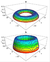
Figure 3 Velocity profiles obtained from simulations (symbols) of axial flow between coaxial cylinders with radii R1 = 8ª and R2 = 16a. Case a corresponds to parameters ® = 180±, P 0 = 0:4, and ·I = ·II = 0:56, these latter were taken from the estimations carried out in Ref. 1. In the case b, these parameters took the values ® = 135±, P 0 = 1:0, and ·I = ·II = 0:56. In both situations a very good agreement is found with the hydrodynamic flow predicted from Eq. (5) (continuous surfaces), where no-slip boundary conditions are assumed. 

Table 1 Experiments proposed to test the validity of the simulation method at different Reynolds numbers. The error parameter " quantifies the deviation of the experimental results from the hydrodynamic flow and is defined by Eq. (9). All quantities are given in simulation units. 

We will use the Reynolds number, Re, in order to characterize the hydrodynamic regime where our simulations are carried out. Recall that Re quantifies the relevance of the inertial forces with respect to the viscous effects. For flow between coaxial cylinders, Re takes the form

where 𝑣 𝑧 is the average flow velocity along the long axis and 𝐷 𝐻 =2 ℛ 2 − ℛ 1 , is the so-called hydraulic diameter. In our case, 𝑣 𝑧 can be calculated directly from the simulation results, which allows us to estimate Re for each produced flow.

We conducted four additional simulations designed to test the performance of the proposed method for simulating the expected hydrodynamic flow at different values of Re. In these experiments, we considered systems having the same size and density as those used previously, while the parameters 𝛼 and 𝑃 ′ were selected as it is shown in Table 1, in order to produce flows with Reynolds numbers in the range delimited by the values Re≳1, and Re∼ 10 2 . The specific values of Re obtained experimentally are also presented in Table 1. In order to quantify the deviation of the simulated profile with respect to the expected hydrodynamic flow, we introduce the error parameter, 𝜀, defined as

where 𝑣 𝜆 represents the 𝑧 component of the flow obtained from the numerical experiments, and 𝑣 𝜆 (h) is the corresponding theoretical value for no-slip boundary conditions, obtained form Eq. (5). In these definitions, the subindex 𝜆 is used to indicate the position where flow is measured and calculated, e.g., the location of all the symbols in Figs. 3a and b.

The results of the numerical experiments, summarized in Table 1, show that for a rather wide range of flows characterized for Reynolds numbers that spread over three orders of magnitude, our approach is able to reproduce the hydrodynamic flow in a very satisfactory manner, since the error parameter is found to take rather small values 𝜀≤0.5%.

4. Simulation of azimuthal flow

We will consider now the case where the force acting on the confined MPC fluid does not have axial component. In particular, we will study the flow produced when the MPC particles are subjected to a force field of the form

where 𝑒 𝑖,𝜙 represents the unit vector in the azimuthal direction of the usual cylindrical coordinate system. Notice that, contrary to the case of the unit vectors of the Cartesian basis, 𝑒 𝑖,𝜙 is position-dependent. Therefore, is has been identified with the subindex 𝑖.

In Eq. (10), 𝐹 𝑖,𝜙 denotes the magnitude of an external field acting on each confined particle along the azimuthal direction. A symmetric case that could be of interest, is that of azimuthal forces of the form

where 𝒯 is a constant. This field has the property of exerting a constant torque on the MPC particles that has precisely the magnitude 𝒯. Consequently, it could be anticipated that it will produce an azimuthal symmetric flow between the coaxial cylinders. In the present section we will show that this is indeed the case.

However, before we proceed with our analysis, it is worth noticing that the application of the force field given by Eqs. (10) and (11), will also produce a non-uniform mass distribution in the system due to the centripetal force associated with the azimuthal flow. The results of our simulations will show that, for small values of 𝐹 𝑖,𝜙 , this effect is not significant and that, under such condition, the simulated MPC fluid can be considered to have a uniform density.

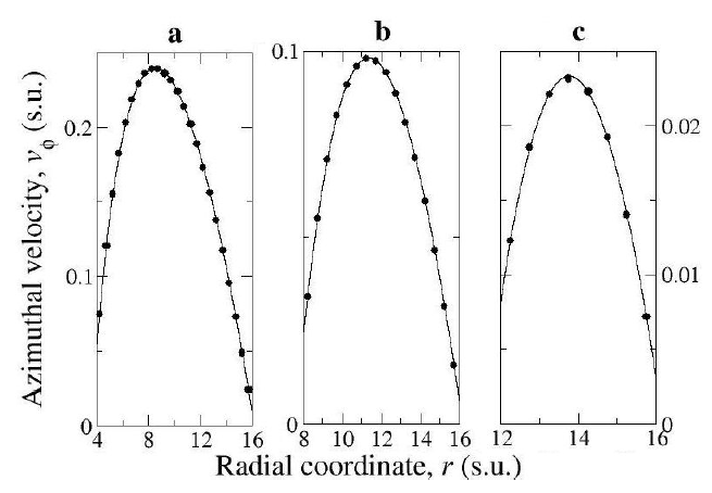
Figura 4 Velocity profiles obtained from simulations (symbols) of azimuthal flow between concentric cylinders of radii R1 = 4a and R2 = 16a (a), R1 = 8a and R2 = 16a (b), and R1 = 12a and R2 = 16a (c). Continuous curves are numerical fits obtained with the general hydrodynamic solution, Eq. (12). In these simulations, virtual particles were introduced with zero mean velocity. Partial slip is observed at the confining boundaries. 

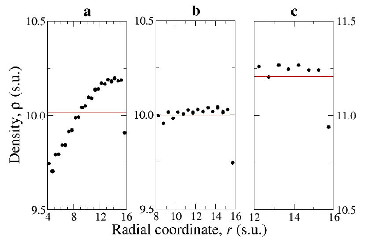
Figura 5 The same as in Fig. 4 for the density profiles obtained from simulations (symbols). Continuous lines represent the average density in each simulated system. 

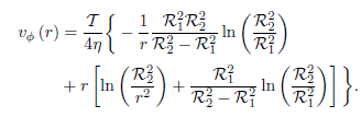
In this case, the general solution of the hydrodynamic equations , can be shown to be

where 𝑎 1 and 𝑎 2 represent integration constants. Equation(12) is supplemented with the conditions of having uniform density and temperature, and observing neither radial

nor axial flow, i.e., 𝑣 𝑟 = 𝑣 𝑧 =0. For arbitrary values of 𝑎 1 and 𝑎 2 , Eq.(12) could be used for describing flow with partial-slip boundary conditions. For the special case of no-slip boundary conditions, we have to impose the equalities 𝑣 𝜙 ℛ 1 = 𝑣 𝜙 ℛ 2 =0, and Eq.(12) takes the form

(13)

Recall that, in our simulation scheme, the transition from partial-slip to no-slip boundary conditions, i.e., the establishment a flow given by Eq. (12) or by Eq. (13), will be controlled by changing the velocity with which virtual particles are introduced at the collision step. In order to emphasize this point and the role that virtual particles play in the case of azimuthal flow, we performed three initial simulations in which these particles were introduced with zero mean velocity. In these experiments, we kept the following parameters fixed: 𝛼= 135 ∘ , 𝒯=0.25, ℛ 2 =16 𝑎, and 𝐿 𝑧 =32𝑎. The first, second and third experiments of this series were performed in systems of different sizes by selecting, respectively, ℛ 1 =4𝑎 and 𝑁=245,760; ℛ 1 =8𝑎 and 𝑁=196,608; and ℛ 1 =12𝑎 and 𝑁=131,072. The values of the total number of particles were selected to yield systems with similar densities ( 𝑛 𝑐 =10.02, 𝑛 𝑐 =10.00, and 𝑛 𝑐 =11.21, for each respective case, where 𝑛 𝑐 denotes the average number of particles per MPC cell).

The azimuthal flows resulting from these simulations are shown in Figs. 4 a, b and c. The velocity profiles presented in this figure were obtained as an average performed over the number of particles contained in coaxial cylindrical sections of radial width 𝑎/2, as well as over the simulation time after thermalization. The continuous curves were obtained after a nonlinear fitting procedure using Eq. (12) as reference and 𝑎 1 , 𝑎 2 and 𝜂 as adjustable parameters. The agreement between the simulation results (symbols), and the hydrodynamic theoretical flow is remarkable.

It is also interesting to present the measurements of the density profiles established in the simulated systems, for the three experiments described previously. These results are shown in Figs. 5 a, b and c, where it can be observed that, as expected, the centripetal force causes a variation of the mass density, 𝜌 𝑟 , through the system. This variation is such that regions at farther distances from the symmetry axis have larger densities. This situation is more clearly illustrated in case a in Fig. 5, that corresponds to a simulated system with size ℛ 1 =4 𝑎 and ℛ 2 =16 𝑎. However, notice that even in this case, changes in density are rather small (<3.0%). Thus, it can be expected that if simulations parameters are kept within this range, the density field can be considered to be uniform and a comparison of the simulated field with Eqs. (12) and (13), will be valid as a first approximation.

Table 2 Numerical estimations of the parameters ·I and ·II that can be used as described by Eq. (14) to produce azimuthal flow with no-slip boundary conditions. All quantities are given in simulation units. 

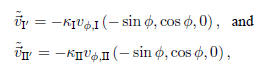
We will consider now the results obtained in experiments performed by introducing virtual particles with average velocities different from zero. It is suggested by the results presented in Fig. 4, that virtual particles should have an azimuthal velocity opposing to that of the fluid, since, in this way, the collision process between real and virtual particles will tend to cancel the flow existing close to the confining surfaces. In order to introduce virtual particles according to this idea, we first calculated the azimuthal average velocity of the particles in the regions I and II described in Fig. 2. Let 𝑣 𝜙,I and 𝑣 𝜙,II , represent such average velocities, respectively. Then, the center of the distribution for the velocities of the virtual particles in regions I ′ and II ′ in the same Fig. 2, was respectively defined by

(14)

where 𝜙 denotes the azimuthal angle associated with the position of the introduced particle. As before, 𝜅 I and 𝜅 II in Eq. (14) are adjustable parameters.

We carried out diverse experiments using trial values of 𝜅 I , 𝜅 II >0, that allowed us to confirm that when virtual particles are introduced according to the rule given by Eq.(14) the slip at the confining cylinders is reduced. We then implemented an optimization procedure analogous to the one used in Ref. 1, in order to find those values of 𝜅 I and 𝜅 II that yield no-slip boundary conditions. Such values are found by imposing the condition that the numerical fit of the simulation results, carried out with Eq. (12), gives velocities lower that 10 −3 when it is evaluated at ℛ 1 and ℛ 2 . Since this procedure is rather expensive from the computational point of view, we restricted our analysis to the case of systems with fixed size and density defined by ℛ 1 =4𝑎, ℛ 2 =8𝑎, 𝐿 𝑧 =32𝑎, and 𝑁=245760. Moreover, we considered only MPC fluids in the liquid-like behavior regime by restricting the collision angle to take large values, 𝛼= 135 ∘ , 150 ∘ , 160 ∘ , 180 ∘ .

We performed the estimations of 𝜅 I and 𝜅 II as function of the collision angle and the external torque 𝒯, that took the values 𝒯=0.05,0.25. The resulting values of the adjustable parameters given by our optimization procedure are presented in Table 2.

It can be noticed from the results presented in Table 2 that the control parameter 𝜅 I seems to be independent of the collision angle and the external torque. Thus, based on the results from our numerical experiments we conclude that, within the range of the simulation parameters considered in our analysis,

On the other hand, 𝜅 II does not change appreciably with respect to 𝛼, but depends on 𝒯. In the simplest case, the function 𝜅 II 𝒯 can be approximated by a linear relation. Using the results of Table 2, we thus have the approximation

With the purpose of verifying the validity of these approximations, we performed a last series of experiments in which the MPC collision angle was allowed to take the values 𝛼= 140 ∘ and 160 ∘ , which were not considered in our previous experiments. In addition, in order to explore the limits of the applicability of Eqs.(15) and (16), simulations were performed using five values of the external torque, 𝒯=0.05,0.25,0.50,0.75,1.00, which extended over values larger than those reported in Table II. The sizes and densities of the simulated systems were the same as those used in experiments from which Eqs. (15) and (16) were obtained. The comparison between the velocity profiles obtained from the last series of experiments and the flow expected from hydrodynamics is shown in Figs. 6 a and b. It is worth stressing that continuous curves shown in Figs. 6a and b correspond to hydrodynamic flow with no-slip boundary conditions, as given by Eq. (13). In evaluating Eq. (13), we estimated 𝜂 by using the average mass density of the simulated system and the general theoretical expressions for the collisional and kinetic contributions to the kinematic viscosity corresponding to our implementation of MPC, see e.g. Eqs. (10) and (11) in Ref. 1. Therefore, the comparison shown in Figs. 6a and b has no adjustable parameters.

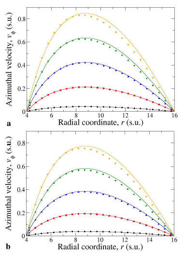
Figure 6 Azimuthal flow between concentric cylinders of radii R1 = 4 a and R2 = 16 a, for two different MPC fluids characterized by the collision angles ® = 140± (a), and ® = 160± (b). Symbols represent the results of numerical experiments carried out with different external torques T = 0:05 (black circles); 0.25 (red squares); 0:50 (blue triangles up); 0.75 (green diamonds); and 1.00 (orange triangles down). Continuous curves represent the flow profile expected from hydrodynamics with no-slip boundary conditions given by Eq. (13). 

It can be observed that the numerical and theoretical results are in an excellent agreement for those values of the external torque contemplated in Table 2, i.e., for 𝒯≲0.25. For larger values of 𝒯, the simulation results do not fit properly the hydrodynamic velocity profile. In fact, deviations appear close to the external cylinder, where flow is smaller than expected. This can be understood since for large torques, density variations could be much larger than those presented in Fig. 5a. In this case, the density and the viscosity of the fluid close to the external cylinder increase and, consequently, flow is inhibited there. Thus, if simulations are desired to approximate an azimuthal flow given by Eq. (13), we recommend to apply the procedure described in the present section by restricting 𝒯 to take small values, 𝒯≲0.25.

5. Conclusions

In this work we have successfully performed simulations of hydrodynamic flow between two coaxial cylinders using MPC. In order to achieve this goal, we have extended the technique based on the use of explicit fluid-solid forces that was originally introduced in Ref. 1. We have described in detail how this technique can be adapted to the specific geometry of coaxial cylinders, with the purposes of confining the MPC fluid and controlling the conditions at the boundary walls. We have considered, separately, the simulation of two kinds of symmetric flows, namely: flows along the axial direction promoted by uniform pressure gradients, and azimuthal flows induced by uniform centrifugal torques. In both cases, our method was able to reproduce the correct hydrodynamic behavior with boundary conditions that could be adjusted from partial-slip to no-slip. Although our simulations of azimuthal flows were restricted to small values of the driving centrifugal forces due the compressible character of normal MPC fluids, it is important to mention that, to the best of our knowledge, simulations of this kind of flows using the MPC technique have not been reported previously in the literature.

There exist many extensions of the present work that could be interesting from diverse standpoints. First, here we have tested the performance of the proposed technique by comparing its results only with those obtained from classical fluid mechanics, although the implementation of an alternative method, e.g., one based on hard-walls, and the subsequent comparison of its computational performance with respect to ours, could be of some interest for researcher in the field of computational physics. Second, in the present paper we have restricted ourselves to analyze the behavior of a pure simple MPC fluid phase. Nevertheless, MPC can be used to simulate colloidal and polymeric suspensions as well. Therefore, an extension of the method introduced here could open the possibility for analyzing the behavior of such complex fluids in centrifugal flow, at least from the point of view of numerical simulations. Finally, it is worth stressing that the analysis carried out here, was limited to show that the proposed method yields results that are in agreement with a macroscopic description of fluid dynamics. However, MPC naturally incorporates spontaneous random forces on suspended particles. Then, another interesting problem could be to analyze of the Brownian dynamics of particles suspended in centrifugal flows, in similar conditions to those that have been recently considered in simpler non-equilibrium scenarios.