


 text new page (beta)
 English (pdf)
 Article in xml format
 Article references
 Send this article by e-mail
 Cited by SciELO
  Similars in
SciELO
Similars in
SciELO 
 Permalink
PACS: 02.30.Hq, 07.50.Ek
1. Introduction
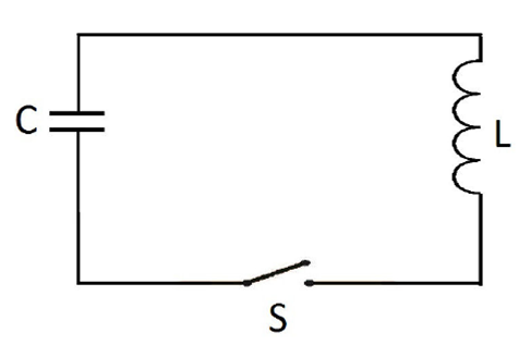
A DC LC circuit in which an inductor (L) and a capacitor (C) are connected to each other is shown in Fig. 1. If the capacitor is initially charged and the switch is then closed, both the current in the circuit and the charge on the capacitor oscillate between negative and positive values. The charge variation of the capacitor with respect to time is defined by a homogeneous second order linear differential equation as follows;
If there is no resistance in the circuit, the standard solution of Eq. (1) is obtained as follows;
where,
In traditional approach where the time scale is considered homogenous, namely, the flow period of time remains unchanged during the physical process (non-relativistic mathematical time), Eq. (1) is local in time and insufficient to take into account the non-conservative nature of physical process. The equations related to the non-conservative systems should be non-local in time. Friction is a well known exemplary for a non-conserved phenomenon and, causes irreversible dissipative effects in the physical processes. As a result of these dissipative effects, time-reversal symmetry is not valid for non-conservative systems. Ohmic friction in the electrical circuits causes the same dissipative effects2,3 . In the literature, in order to compensate these dissipative effects theoretically, the fractional calculus is applied to various electrical circuit problems as a useful mathematical tool4,5,6,7,8,9,10,11,12,13,14,15. In this respect, an approach to design analogue fractional-order controllers was described by Podlubny et al5. An experimental study of two kinds of electrical circuits, a domino ladder and a nested ladder, was presented by Sierociuk, Podlubny and Petras6. Some fractional models used in electrochemical systems7, multivibrator built around a single fractional capacitor8, evolution of a current in a resistor9, fractional linear systems10 and reachability of fractional electrical circuits11 were investigated. The series RLC circuit in the fractional-order domain was studied and, the stability issues for different cases which were required to design the fractional-order filters and oscillators were discussed in Ref. 12. The fractional methods were used to solve problems in conservative and non-conservative oscillatory systems with RL and RLC applications13 . Fractional viscoelastic models were applied to biomechanical constitutive equations . The time fractional differential equation related to electrical RC circuit was solved by making use of Caputo fractional derivative in our previous study15.
Fractional differential equations for RLC and RC-LC circuits in terms of the fractional time derivatives of the Caputo type were proposed in Refs. 16 and 17. To keep the dimensional coherence, a new parameter, σL, was introduced by them 18. This parameter characterizes the existence of fractional structures which emerges from the non-local behaviour of the system in time. In Ref. 17, Eq. (1) is re-defined as follows;
where,
Another study on this subject was carried out by Rousan et al in Ref. 19 where the differential equations related to RC and RL circuits are merged in a single equation as follows;
where,
where, q(0) = q0.
Since the nature of electrical LC circuit is non-linear and non-local in time, Eq. (1) is not qualified to give a realistic description for considered phenomena. To make a description closer to reality, the effects of ohmic friction and temperature (as a physical quantity related to resistance), which cause the non-local behaviours in time, should be taken into account in calculations. Eq. (1) is only a simple description of the LC circuit by ignoring the dissipative effects and fractality of time. Therefore, in order to take into account the fractality of time, time-fractional derivative should be used in Eq. (1). Some studies, which are interested in this problem, can be found in the literature. But, one of them has incorrect oscillation of the fractional solution19 and, some of these studies have used a new parameter to keep the dimensional coherence16,17,18 . In the present study, Caputo definition has been preferred for the time-fractional derivative and, the dimension of time-fractional equation is preserved without using any parameter.
In section two, preliminarily of fractional calculus and the meaning of using time fractional derivative is presented. In section three, the differential equation for LC circuit is solved in a fractional manner and, the charge variation of capacitor with respect to time is obtained in terms of Mittag-Leffler function. In section four, the graph of the charge variation versus time is plotted for the different values of fractional derivative order α. Finally, conclusions have been given in the last section.
2.The Meaning of Using Time Fractional Derivative
Standard mathematical approaches are not sufficient to explain the realistic behaviour of the many physical processes in which the fractal property of space and the non-Markovian nature of statistical phenomena occur. Time-reversal symmetry and time locality, which are valid for conservative systems, fails for the realistic nature of physical processes. In order to account for the time-fractality effects (namely, nonlocality in time, time-irreversibility and, memory effects) encountered in the physical systems, time fractional derivative operators are often used in the course of calculations. Especially, they are very successful in the study of the self-similar, hierarchically organized systems and, the linear response of systems with memory20,21,22,23,24,25,26,27.
Fractional calculus is a branch of mathematics which deals with the generalization of integer-order integration and differentiation and, includes the standard definitions as particular cases. The most commonly definitions used in the literature are Riemann-Liouville, Caputo and Grünwald-Letnikov fractional derivatives4,21,22,25 . The presence of many different definitions of fractional derivative makes possible to be taken additional physical information into account in calculations27.
In this study, as a time fractional derivative, we prefer to use Caputo definition instead of standard time derivative. The left-sided Riemann-Liouville fractional integral of order α is given as follows,
where, α is any positive real number and Γ(α) is Gamma function and, t parameter corresponds to the last measured value of mathematical time. Caputo fractional derivative of order α is given by the definition:
where, m is the smallest integer greater than α, i.e. m -1 < α < m. In physical applications, Caputo definition of fractional derivative is more preferred, other than Riemann-Liouville definition, because it includes the initial values of the function and its integer order derivatives when Laplace transform method is used4,20,21,25.
The solution of fractional differential equations can usually be expressed in terms of the Mittag-Leffler function as a natural generalization of exponential function and, is defined by the series expansion as follows4,21,26:
In the well known differential calculus developed by Newton, time is assumed to have a homogeneous equably flowing nature and, is also specially called “mathematical time” which has no relation to external factors. Indeed, the successfully use of differential calculus in the study of the mechanics of macro-particles is based on the mathematical time assumption. In the view of the Newtonian approach, the total mathematical time consists of geometrically equal time intervals. On the other hand, since the measurement process of time intervals cannot be made at the same time, it is not possible to find an evidence which shows the homogeneity (or equality) of time intervals. According to the current views in relativity theory, time intervals are not absolute physical quantities, but instead they depend on gravitational fields in which the measurements of time intervals are made. The inhomogeneous nature of time is indicated by the term of “physical (or cosmic) time”. The total physical time consists of geometrically non-equal time intervals. As an example, the time flows non-equably for the physical processes handled in relativistic manner28 .
In the time fractional approach adopted by Podlubny, the left sided Riemann-Liouville
fractional integral has been reformulated in the form of Stieltjes integral, namely
In the present study, we know that the amount of current transferred to the circuit varies for each Δt time intervals. If the current being transferred to the circuit at each Δt step is considered to be equal to each other, the width of Δt time intervals may be considered different from each other. When we make such a consideration, the physical reality does not change and, we can say that the physical event considered in this paper exhibits non-local behaviour in time. Therefore, in order to make a more realistic description, time-fractional derivative can be used in the calculations.
3. Analysis of Electrical LC Circuit in Fractional Order
In order to establish a time fractional differential equation which describes the LC circuit, the Caputo fractional derivative of order α is used instead of the first order standard time derivative. Thus, the equation in fractional order is given by
where
In order to obtain a solution, firstly the Laplace transform is performed to Eq. (10) leading to
where,
The inverse Laplace transform of Eq. (12) can be expressed in terms of Mittag-Leffler function,
4.Results and Discussion
Assuming the components of LC circuit have negligible resistance, the variation of capacitor charge with respect to time is obtained as Eq. (2) in course of the standard calculations. According to this solution, the charge of capacitor is not damped, but instead makes oscillation between negative and positive values. However, in realistic frame, the components of circuit have resistance and the variation of charge is damped and, converges to zero with time. In the present study, in order to represent the realistic situation, standard LC circuit equation, i.e. Eq. (1), has been re-defined as Eq. (10) by using time fractional derivative of order α. The solution of this new equation has been obtained in terms of Mittag-Leffler function as Eq. (13). In order to investigate the graphical representations, the values of inductor and capacitor have been taken as L=1H and C =1 F in calculations, respectively.
As seen from Fig. 2, the variation of capacitor charge with respect to time has been plotted by Rousan et al. in Ref. 19 by using Eq. (6). In this figure, q(t)/q 0 values have been calculated for different α values. The standard solution, i.e. Eq. (2), has been indicated with dashed line. As menmentioned in the first section, when α is equal 1, Eq. (5) corresponds to well known differential equation of LC circuit. As seen from Fig. 2, all curves start from origin except the one which corresponds to α = 0. Whereas, at t = 0, the initial values of q(t)/q 0 should be 1. This exhibited behaviour shows that fractional solution is not in harmony with the well known standard solution for α = 1 and, there is a phase difference between the fractional solution and standard one.
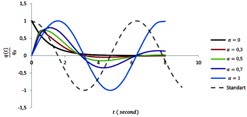
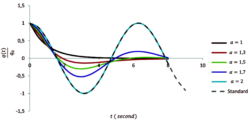
Figure 3, presented in this study via Eq. (13), depicts the charge variation of capacitor with respect to time for different values of α. Unlike Ref. 19, as a time fractional derivative Caputo definition is used in this study. When α = 2, Eq. (10) corresponds to the well known standard differential equation related to LC circuit. In Fig. 3, the standard solution has been indicated with dashed line. For α = 2, a complete harmony between the standard solution and the fractional solution can be seen from Fig. 3. In other words, there is no phase difference between the standard and fractional solutions.
In order to make a realistic description of the considered physical process, the resistance value of the cables connecting the circuit elements to each other should not be handled as a constant parameter, instead it should be considered as a varying physical quantity with temperature. Due to the increase in temperature, the spatial distribution of the charge carriers in cables changes. Hence, the homogeneity of the circuit is impaired and, the structural fractal effects become dominant over time with increasing temperature. As a result, the charge variation of capacitor with respect to time exhibits a damped behaviour. In present study, this exhibited behaviour is clearly described with the use of fractional derivative of order α which varies between 1 and 2. Hence, the structural fractal effects, occurred in the LC electrical circuit due to the temperature, can be taken into account in the calculations. From these results, it could be said that there is a close relationship between the temperature and fractional derivative of order α.
5. Conclusion
A new time-fractional form of the differential equation related to electrical LC circuit is determined as Eq. (10). In this equation, different from Refs. 16 to 18, dimensional coherence are preserved without using any parameters.
Equation (1), used in standard approach, corresponds to ideal case in which the dissipative effects are neglected. Therefore, LC circuit is handled linear and local in time. In realistic manner, the resistance of the cables connecting the circuit elements to each other varies with the temperature. This unstable resistance causes some dissipative effects which make the behaviour of LC electrical circuit be non-linear and non-local in time. Since the temperature of LC circuit increases with time, an unstable ohmic friction occurs during the process. Also, in a real capacitor series resistance is not zero and in the parallel resistance is not infinite. The series resistance in an inductor is not zero. Hence, the current transmitted to circuit (and also the charge variation of the capacitor) per each small time interval (Δt) exhibits a difference in each Δt step. Hereby, time reversal symmetry for this process is not valid. From a different perspective, to indicate the nonlocality in time, the transmitted current can be assumed being unchanged per different time intervals Δt and, the flow period of Δt intervals can be assumed being variable depending on the temperature. Consequently, it could be said that using the time fractional derivative instead of standard one is a very useful way to describe the realistic feature of LC electrical circuit that is non-local in time.

