


 nova página do texto(beta)
 Inglês (pdf)
 Artigo em XML
 Referências do artigo
 Enviar este artigo por email
 Citado por SciELO
  Similares em
SciELO
Similares em
SciELO 
 Permalink
PACS: 42.81-I, 42.81Gs; 42.25.Ja
1. Introduction
In single-mode fibers, internal perturbations such as core or cladding asymmetries and internal stress produce characteristic differences of the propagation constants of the orthogonal polarization modes. Although these contributions can be considered to vary randomly for long fiber lengths (km), it is clear that a few meters straight fiber presents a uniform structure. As absorption is usually negligible, it is commonly assumed that the fiber behavior corresponds to that of a homogeneous retarder whose polarization properties are often described only by the phase evolution caused by birefringence, characterized by the polarization beat length Lb . Polarization beat length can be easily measured using Jones calculus, a null linear polariscope and either the cut-back method 1, or the wavelength scanning technique 2. It is important to acknowledge that this type of evaluation is complete only when the residual birefringence is linear and the azimuth angle of the fast birefringence axis is known or when it is circular.
The characterization of the input and output states of polarization does not supply enough information on the birefringence parameters of the fiber 3. To build the birefringence matrix it is also necessary to determine the azimuthal and elliptical angles of the fiber anisotropy. This can be accomplished mapping the evolution of the polarization states along the fiber. This procedure is frequently avoided because it requires the use of a more complex optical arrangement and time-consuming data processing. The evolution of light polarization along the fiber should be plotted using either the polarization complex-plane or the Poincaré sphere 4,5.
In addition, it is important to mention that recently it was shown that the fiber might also present residual torsion 6, an additional uniform contribution that is typically neglected. Its relevance relies on the fact that in the presence of torsion the fiber no longer behaves as a homogeneous retarder 7,8. Its birefringence corresponds to a homogeneous retarder followed by a rotator 9 and the evolution of the state of polarization is no longer periodic.
This work is organized as follows. The measurement of the polarization retardation rate, characterized in terms of the polarization beat length, and the type of results that can be obtained using the widely applied procedure based on intensity measurements and Jones calculus are presented in Sec. 2. To avoid a priori assumptions on the fiber birefringence we consider it is necessary, to identify the type of anisotropy present in our sample. Therefore, polarimetric procedures used for this purpose are shown in Secs. 3 (homogeneous retarders) and 4 (twisted homogeneous retarders). Section 5 contains our conclusions.
2. Polarization Beat Length Identification
In this work it is assumed that the fiber presents a negligible absorption. Under these circumstances, the change introduced by the fiber birefringence does not affect the signal power, there is just a phase retardation between the polarization eigenmodes. When the fiber behaves as a homogeneous retarder and the phase change is δb = 2π, the input state of polarization is restored at the fiber output; the length L = Lb (polarization beat length) associated to this phase change is used to evaluate the retardation rate of change of the fiber birefringence.
The measurement of the polarization beat length is performed using a null polariscope, a very simple low cost arrangement, in which the changes introduced by a birefringent sample on the light’s polarization state are shown as intensity variations. Using this instrument it is possible to follow the evolution of the polarization state along the sample applying the cut-back or the wavelength scanning technique, and as we shall show below, the type of retarder and the azimuthal angle of birefringence can be identified.
2.1 Null Linear Polariscope
In the null linear polariscope shown in Fig. 1, light from a monochromatic light source is linearly polarized and launched into a sample of single-mode fiber using a microscope objective. The light emerging from the far end of the fiber is collimated using another objective and passes through the analyzer before reaching the detector.
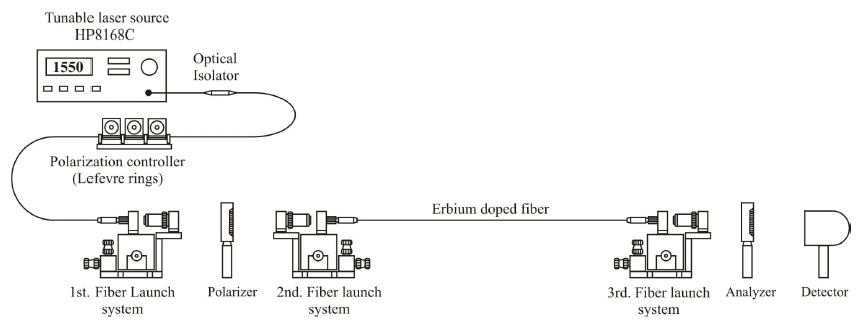
FIGURE 1 Null polariscope. The monochromatic signal comes from a tunable diode laser. A polarization controller and a microscope objective are used to produce collimated circularly polarized light to illuminate the input polarizer. Microscope objectives are used to couple light to the single-mode fiber and to collimate it at the fiber output.
To determine the trajectories we would observe for polarization evolution in each type of homogeneous retarder, matrix calculus can be used. When an input linear polarization signal Ein is launched into the fiber, at its rear end the output polarization state (Eout) is given by,
where the linearly polarized input signal with azimuth angle φ can be written as
in terms of the Jones vector Ein, or as
in terms of the Stokes vector Sin (using a simplified 1×3 notation), and M is the fiber birefringence matrix.
In general, when the straight fiber sample is placed between the input polarizer and the analyzer, its fast birefringence axis is not aligned with the polarization axis of the input linear polarizer. For simplicity we assume that the birefringence axis of the fiber is aligned with the laboratory reference frame, while the polariscope axis is rotated an angle φ. In this case, using Jones calculus, the electric field at the polariscope output is
where P
φ
and
and M is the Jones matrix of the fiber sample.
2.2 Measurement of the Polarization Beat Length
In what follows we calculate the intensity at the polariscope output considering that the length of the optical fiber is modified (cut-back method) or the wavelength of the sampling signal is scanned (wavelength scanning method). It is important to mention that in both cases, to avoid the contribution of dispersion, the light signal used for each measurement must be a monochromatic signal, and for wavelength scanning, it is also necessary to verify that within the range of measurement birefringence dispersion is negligible.
2.2.1 The fiber behaves as a homogeneous retarder
To describe the fiber anisotropy we use the birefringence matrices associated to anisotropic media whose fast birefringence axis lies on the x axis (azimuth angle α = 0). Jones matrices are shown in Table I, and in Table II we present simplified 3 × 3 Mueller matrices 11. In this work we use a right hand matrix to describe the elliptical retarder 12.
TABLE I Jones matrices of the retarders used to describe the bire- fringence of single-mode fibers 10.
It should be noticed that we decompose the polarization vector in terms of polarization eigenmodes. This eigenmode of the state of polarization (SOP) of light as it evolves along the fiber, the light’s SOP is described in terms of the normal modes associated to this oscillation: two orthogonal unitary vectors (see 5). Since polarization eigenmodes are normal modes, when light is launched in one of these polarization states, its SOP remains unchanged while propagating along the fiber.
For both sets of matrices it is clear that the matrix of an elliptical retarder corresponds to the general case, being particular cases the linear retarder (ε = 0) and the circular retarder (ε = π/4). The retardation introduced by the fiber birefringence does not modify the signal power. It only introduces a phase change between the polarization eigenmodes that can be described as
where Δn is the birefringence (linear, circular, or elliptical), λ the signal wavelength and L the fiber length. It is clear from Eq. 12 that using the cut back method or the wavelength scanning technique the evolution of the polarization state along the fiber can be followed. In this section it is assumed that the birefringence of the fiber sample is uniform and is either: linear, circular, or elliptical (Table I). Using equations 1, 2, 5 and the proper Jones matrix from Table I in relation 4, it can be shown that for each type of retarder the linear output state of polarization is aligned with the analyzer polarization axis, and its intensity is given by the expressions shown in Table III.

When the angle between the sample birefringence axis and the polariscope axis φ is equal to 45°, Eqs. 13 to 15 are equal to
To relate equation 16 with the polarization beat-length of the fiber we use Eq. 12,
When the azimuth angle of the polariscope is φ ≠ 54°, the amplitude of the curve (Fig. 2) decreases, but according to equations 13 to 15, the locations of maxima (or minima) along the fiber length used to evaluate the polarization beat length, do not displace. Therefore, using this simple experimental procedure, one fiber orientation with respect to the null polarimeter (φ), and considering the fiber length required to obtain three maxima (or minima) we can evaluate the polarization beat length (vertical line in Fig. 2).
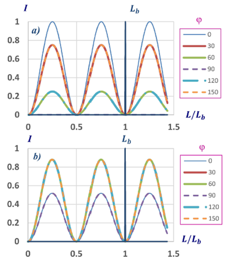
FIGURE 2 Null polariscope output for a fiber whose beat-length is Lb. a) linear retarder, b) elliptical retarder with ε = 23◦. In both cases the azimuth of the input linear polarization state is different for each curve (φ), it varies from 0 to 150◦. The output intensity presents a higher amplitude modulation for azimuth angles of the signal’s input polarization state close to the azimuth angle of the fiber’s fast axis (φ = 0◦).
As we can notice in Fig. 2, the curves obtained for the output intensity evolution are similar for linear and elliptical retarders, therefore using only one azimuth angle for the input linearly polarized signal we do not have enough information to be able to discern if the homogeneous retarder that can be used to describe the fiber anisotropy is linear or elliptical.
2.2.2 The fiber presents a residual torsion
The birefringence matrix of a fiber with homogeneous retardation and residual torsion τ is 7:
where β and b are constants. It has been demonstrated in 6 that the fiber birefringence exhibits, as a cold twisted fiber, a geometrical contribution introduced by the rotation of the birefringence axes and described by the matrix R(β + bτ), and a photoelastic contribution. Matrix Mτ is the matrix of a homogeneous retarder whose retardation angle δ τ in addition to the retardation δi associated to homogeneous retardation, presents a linear dependence with the residual torsion, introduced by photoelasticity
where c is a photoelastic constant Eq. 19 can be rewritten in terms of the fiber length L as
where pi = δi /L is the propagation constant associated with δi , ρ = τ/L is the twist rate per unit length and g is a constant. This relation is similar to that obtained in Ref. 13, but as we can notice, g is different from Ulrich constant.
For linear and elliptical retarders, in Eq. (18) we have two rotations about different gyration axes; therefore the fiber behaves as a non-homogeneous retarder 8. It will behave as a homogeneous retarder only if the retarder is circular.
It is possible to determine the output intensity dependence on length, for a fiber that behaves as a linear, circular or elliptical retarder with residual torsion, using Eqs. (1), (2), (18), (19), (5) and the proper Jones matrix in Eq. (4). The relations obtained are shown in Table IV.

When a linear retarder with residual torsion is inserted in a null linear polariscope, we can see again that the amplitude modulation of the output intensity is maximum when φ = 45°, but as we can see in the examples of Fig. 3, the amplitudes of maxima and minima of intensity are not constant. In addition, the shape of the output intensity curve is periodic only when δ τ/θ is equal to a rational number (Fig. 3(b)). Therefore we can speak of polarization beat length only in this case.
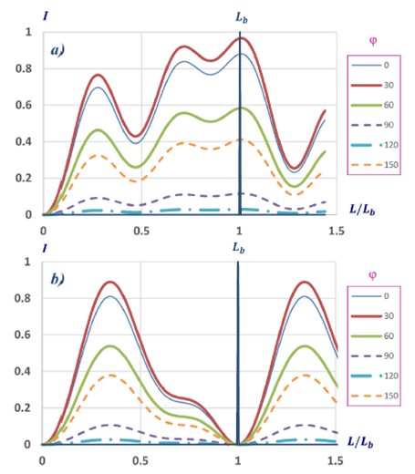
FIGURE 3 Null polariscope output for a linear retarder with residual torsion. The azimuth (φ) of the input linear polarization state is different for each curve (0 - 150◦). The relative values of the retardation angle δτ and the rotation angle θ are different: a) δτ = 4.2θ; b) δτ = θ.
In Fig. 3(a) we have marked the position where the phase retardation δ τ is equal to 2π with a blue line. It is evident that the input polarization state is not reproduced for that fiber length. For Fig. 3(b) we also used a vertical line to mark the position where δ τ = π; i.e., L = Lb /2. We can notice that in this case we will also require three minima to obtain a length increment equal to one polarization beat length.
We present in Fig. 4 two additional examples of the output intensity profiles, obtained in this case for an elliptical retarder with residual torsion. The elliptical retardation is ε = 23° and the azimuth angle of the polariscope is φ. In this figure we present the evolution obtained for different relative rates of the retardation and rotation angles, δ τ/θ = 4.2 (Fig. 4(a)) and δ τ/θ = 1 (Fig. 4(b)). We can observe again that when this ratio is not equal to a rational number the evolution is not periodic.
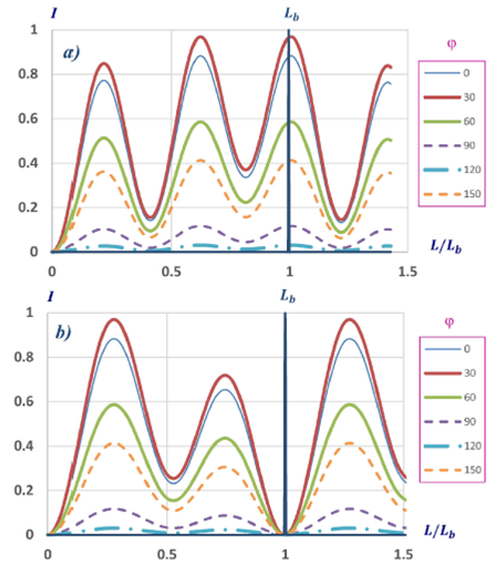
FIGURE 4 Null polariscope output for a fiber that behaves as el- liptic retarder (ε = 23◦) with residual torsion. In both cases the azimuth of the input linear polarization state φ, is different for each curve, it varies from 0 to 150◦. a) δτ = 4.2θ; b) δτ = θ.
From Eq. (18) it is evident that a periodic evolution of the output intensity along the fiber can be obtained applying a proper twist to the fiber (the value of the ratio δ τ/θ is modified). Therefore, as it has been suggested 14, twisting a fiber can be used to get a more stable evolution of light polarization.
In regard with the rate of change of the retardation angle δ τ, when the polarization evolution of light along the fiber is periodic we can still talk about a polarization beat length and measure it considering three consecutive minima.
In order to visualize the relevance of the rotation angle θ associated to the rotation of the birefringence axes produced by torsion, we varied the ratio δ τ/θ keeping the same rate of change for δ τ. The results are shown in Fig. 5. In Fig. 5(a), the ratio δ τ/θ is equal to 1/2 and in Fig. 5.b, to 1/3. We can see that the prediction for the polarization beat length produces the same value. Therefore, introducing a cold twist we can produce a ratio δ τ/θ that corresponds to a rational number and evaluate the polarization beat length of the linear or the elliptical retarder that presents a residual torsion14. Furthermore, we can notice from figures 4.b and both graphs in Fig. 5 that the number of maxima indicate the relation between δ τ and θ.
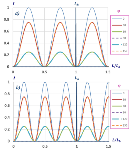
FIGURE 5 Null polariscope output for a fiber that behaves as linear retarder (ε = 0◦) with residual torsion (θ = angle per unit length). In both cases the rate of change of δτ is the same and the azimuth of the input linear polarization state (φ) varied from 0 to 150◦. a) δτ = 2θ; b) δτ = 3θ.
We can see from Figs. 4 and 5 that the output intensity measured for the maxima is higher when the azimuth angle of the fast birefringence axis of the fiber is aligned with the polariscope (φ = 0).
2.3 Birefringence Identification Using a Linear Polariscope
In this section we use the results of the previous section to identify the type of retarder that describes the birefringence of the single-mode fiber under evaluation. From Eqs. (13-15) we can notice that for a circular retarder the output intensity does not depend on the orientation of the fiber; while for linear and elliptical retardations the output intensity is modified by the orientation of the sample with respect to the linear polariscope. We can see from Eq. (13) that when the linear retarder is aligned with the polariscope, i.e. when φ = 0° the output intensity for all values of L (or λ) is null. While, Eq. (15) indicates us that varying the relative orientation of the fiber sample with respect to the polariscope we cannot reach this condition for any value of φ. Therefore, using these different responses to the relative orientation of the sample with respect to the polariscope and the azimuth angle of the input linear polarization we can identify the type of homogeneous retarder that describes the fiber birefringence.
When the fiber presents a residual torsion, the relation that describes the output intensity variation with length for a linear (Eq. 21) or elliptical retardation (Eq. 23) is not homogeneous. The profile of the output intensity curves presents a non-uniform oscillatory behavior, periodic only in some cases. As we mentioned above, when the residual birefringence does not produce a periodic profile, it can be modified to reach this condition introducing a cold twist (by trial and error). Under this condition it is possible to measure the polarization beatlength and the relative rate of change of the retardation between polarization eigenmodes to the twist angle of the total torsion. Analyzing the profile variation of the evolution of the output intensity for different azimuth angles of the input linear polarization it is also possible to distinguish between linear and elliptical retarders.
3. Polarization Eigenmodes Identification (Homogeneous Retarder)
To be able to build the birefringence matrix, it is necessary to determine the values of the azimuth and ellipticity angles that characterize the polarization eigenmodes. In this section we consider initially that the fiber behaves as a homogeneous retarder and incorporate the contribution of residual torsion in Sec. 4. In both sections, we present two alternatives for the identification of the homogeneous birefringence present in the fiber and the determination of their elliptical and azimuthal angles. When the polarization states are described in terms of Jones vectors, data of the polarization evolution along the fiber length are analyzed plotting the resultant trajectories on the polarization complex-plane 4. If Stokes vectors are used to describe the output polarization states, the analysis is performed mapping the polarization evolution on the Poincaré sphere 5. A third alternative with a higher accuracy can be used only when the fiber behaves as a homogeneous retarder 15.
3.1 Polarization Complex-Plane Representation
It has been demonstrated that when the Jones matrix formalism (Eq. 2 and matrices of Table I) is used to describe the evolution of the light polarization state along the fiber, the results, plotted on the polarization complex-plane produce circular trajectories 4. We present in Table V the locus of the center of curvature and the radius of curvature, obtained for the trajectory of each type of homogeneous retarder on the polarization complex-plane.
TABLE V Radius and center of curvature of the trajectories on the polarization complex-plane representing the evolution along the fiber of a linear input SOP.

In the complex-plane of polarization the polarization states are represented using the real and imaginary parts of the quotient between the y and x components of the electric field vector. The real part of Ey /Ex is associated to the horizontal axis (u) and the imaginary part, to the vertical axis (v). This representation is a projection of the Poincaré sphere on a plane 10.
Using simplified Mueller matrices (Table II) and Stokes vectors (Eq. 3) it has also been shown that the evolution of the light polarization state along the fiber mapped on the Poincaré sphere produces circular trajectories 5. The resultant circles are perpendicular to a common line of symmetry, and it can be shown that the intersections of this line of symmetry with the Poincaré sphere [(2α, 2ε)and the orthogonal position, (2α + π, 2ε + π) ] indicate the location of the polarization eigenmodes. The Poincaré sphere is a unitary double sphere where the azimuthal and elliptical angles are described using the double of its real value.
3.2 Graphical Analysis for Eigenmodes Identification
3.2.1 Homogeneous linear retarder
When the fiber behaves as a linear retarder, and the complex-plane representation is used, the center of curvature lies always on the real axis. This indicates that the ellipticity angle is ε = 0, as we can see from the relation for the position of the center of curvature shown in Table V. From Eq. (24) we can see that using an input signal with azimuth angle φ = 0
therefore, Eq. (26) can be used to determine the azimuth angle α of the linear retarder.
When the Poincaré sphere is used, we know that the fiber behaves as a linear retarder when the intersection of the symmetry axis of the circular trajectories with the Poincaré sphere is located on the equator. In this case the ellipticity angle ε is null, and the azimuth angle of the linear retarder is equal to the semi angle between the symmetry axis of the circular trajectories and S1 axis.
Examples of the curves we can obtain for the evolution of a linear input SOP along a fiber that behaves as a linear retarder are presented in Fig. 6. Figure 6(a) contains the trajectories plotted on the polarization complex-plane when the fiber fast birefringence axis forms an angle α = 30° with the horizontal axis. In Fig. 6(b) the trajectories mapped on the Poincaré sphere correspond to a linear retarder with azimuth angle α equal to zero. In both cases when δ > 2mπ (m is an integer), the next circular trajectory reproduces the previous one.
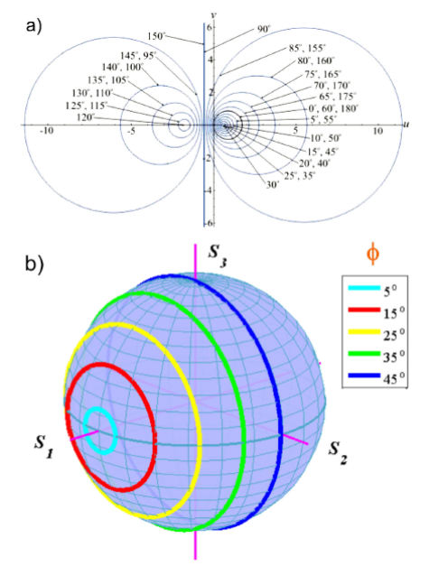
FIGURE 6 Linear retarder. a) The fast birefringence axis forms an angle α = 30◦ with the horizontal axis. Each curve corresponds to a different azimuth angle φ of the input linearly polarized signal (0 < φ < 180◦). b) The fast birefringence axis coincides with the horizontal axis. Each circle corresponds to a different azimuth angle φ of the input linearly polarized signal (0 < φ < 45◦; 10◦ step).
3.2.2 Homogeneous circular retarder
The identification of a circular retarder is easy in both cases. When the polarization complex-plane is used, the trajectory of a linearly polarized input signal evolves along the real axis (horizontal axis) in the positive or negative direction, depending upon the sign of the retardation (right- or left-handed circular retarder). On the Poincaré sphere, the trajectory of a linearly polarized input signal evolves along the equator, also in the positive or negative direction for right- or left-handed circular retarders, respectively.
3.2.3 Homogeneous elliptical retarder
In this case, for a linearly polarized input signal the circular trajectories depicted on the polarization complex-plane are not centered on the horizontal axis, as we can see from the expression for (ue,ve ) in Table V. We can also notice from this relation that when the azimuth angle of the input linearly polarized signal is null (φ = 0°),
Using Eq. 27 we can determine the values of the azimuth angle α, and the ellipticity angle ε of the fiber’s anisotropy.
Examples of the circular trajectories predicted for elliptical retarders are shown in Fig. 7. For the complex-plane representation, the centers of the circular trajectories lie on the imaginary axis (vertical axis) when the azimuth angle of the fiber anisotropy α is zero (Fig. 7(a)). When the fast birefringence axis of the fiber anisotropy forms an angle with the horizontal axis of the measurement system (α ≠ 0), we can see in Fig. 7(a) that the centers of the circular trajectories are located on a straight line forming an angle ξ with the real axis (horizontal axis), whose value according to Eq. 27 depends both on the ellipticity and the azimuth angle of the fiber elliptical birefringence, ξ = arctan(tan2ε/sin2α).
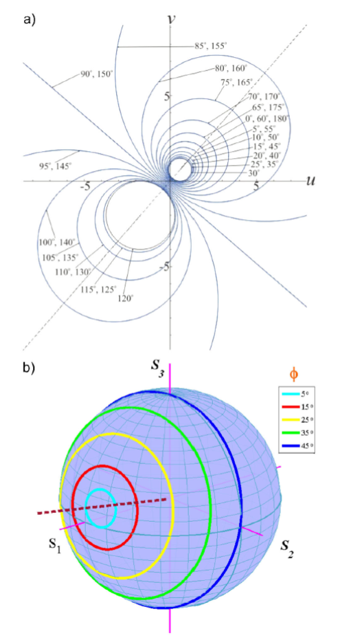
FIGURE 7 Elliptical retarder. a) Ellipticity angle ε = 22.5◦, azimuth angle α = 30◦. Each curve corresponds to a different azimuth angle φ of the input linear polarization signal (0 < φ < 180◦). b) Ellipticity angle ε = 5◦, azimuth angle α. Each curve corresponds to a different azimuth angle φ of the input linear polarization signal (0 < φ < 45◦; 10◦ step).
When the Poincaré sphere mapping is used, the intersection of the axis of symmetry of the circular trajectories with the Poincaré sphere indicates the values of the azimuth angle α (horizontal semi angle along the equator, measured from axis S1) and the ellipticity angle ε (vertical semi angle measured from the equator).
3.3 Eigenmodes Identification Using a Monochromatic Signal and the Poincaré Sphere
For the evaluation of the fiber birefringence this procedure uses a single monochromatic signal 15, therefore its precision is not affected by birefringence dispersion. It is based on the geometric properties exhibited by retarders when the polarization evolution of light is mapped on the Poincaré sphere.
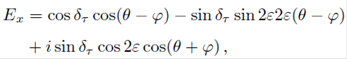
When the fiber behaves as a homogeneous retarder, for any linearly polarized input signal, the light state of polarization traces a circular path on the Poincaré sphere having as center of symmetry an axis whose intersection with the Poincaré sphere has angular coordinates (2α, 2ε). Therefore, angles α and ε, the azimuthal and elliptical angles of the fiber birefringence, can be determined using the circular evolution of the input linear polarization along the retarder 16. In what follows, using Fig. 8 we describe the experimental procedure applied to the characterization of an elliptical retarder (general case of a homogeneous retarder). When the output polarization becomes linear (αl -out), its azimuthal position along the equator is symmetrical with that of the input linear polarization (αl -in), with respect to the azimuthal position of the closest polarization eigenmode (2α). Therefore,
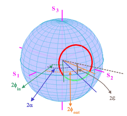
FIGURE 8 In the Poincare´ sphere, the evolution of the state of polarization of light describes a circular trajectory perpendicular to an axis of symmetry that intersects the sphere at the fiber polarization modes.
Once we have determined the value of the azimuth angle of the fiber birefringence (α), we can calculate the values of the Stokes parameters S1 and S2 that correspond to this position and determine, using a polarization analyzer, the maximum and minimum values of the Stokes parameter S3 for this azimuthal position. We denote the maximum and minimum values of the ellipticity angle for this trajectory as:
4. Polarization Eigenmodes Identification in the Presence of Residual Torsion
4.1 Complex-Plane Representation of Homogeneous Retarder with Residual Torsion
Assuming the general case of an elliptical retarder, using the Jones representation, the components of the output electric field are:
 (30)
(30)
 (31)
(31)
where θ = β + bτ. And the components along the real and imaginary axes of the polarization complex plane are:
 (32)
(32)
 (33)
(33)
4.1.1 Linear retarder with residual torsion
The case of a linear retarder corresponds to an ellipticity ε = 0. In this case, from Eqs. 32 and 33 we obtain
 (34)
(34)
 (35)
(35)
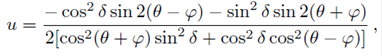
Examples of the results we obtain for a linearly birefringent fiber with residual torsion are shown in Fig. 9. We can see that the trajectories are not circular and their shapes also show a strong dependence on the azimuth angle of the input polarization state. Consecutive loops have a different shape and they overlap only when δ τ/θ is equal to a rational number 17. In Fig. 9(a)δ τ = 4.2θ, while in Fig. 9(b) the closed curves we observe are formed when the rotation angle is equal to the retardation angle of the elliptical retarder with residual torsion (δ τ = θ).
FIGURE 9 Trajectories of the polarization evolution of light along a linearly birefringent fiber with residual torsion, represented on the polarization complex-plane. a) δτ = 4.2θ (open curves). b) δτ = θ; in this case we obtain closed trajectories. In both figures the linearly polarized signals have different azimuth angles (20, 40, 80 and 120 degrees). Using the same order, trajectories are shown with: blue, green, red and light blue lines.
4.1.2 Circular retarder with residual torsion
In this case the fiber behaves as a homogeneous retarder, therefore the results follow the behavior reported for a circular retarder without residual torsion (Sec. 3.2.2).
4.1.3 Elliptical retarder with residual torsion
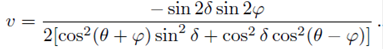
Examples of the type of plots we obtain for an elliptically birefringent fiber with residual torsion are shown in Fig. 10. The values we used for the retardation rates are the same as those used for the examples in Fig. 9. We can see that in this case the trajectories are no longer circular and their shapes show a strong dependence on the azimuth angle of the input polarization state. In general, when the retardation δτ is larger than 2mπ (where m is an integer), consecutiveloops have a different shape, they overlap only when δτ / θ is equal to a rational number 17 (we should remember that this representation is a projection of the Poincaré sphere on a plane). In Fig. 10(a) the rotation angle θ is smaller than the retardation angle δτ (δτ = 4.2θ), while in Fig. 10(b) the closed curves we observe are formed when the rotation angle is equal to the retardation angle of the elliptical retarder with residual torsion (δτ = θ).
FIGURE 10 Trajectories of the polarization evolution of light along an elliptically birefringent fiber with residual torsion, represented on the polarization complex-plane. a) δτ = 4.2θ; these are open curves b) δτ = θ; in this case we obtain closed trajectories. In both figures the linearly polarized signals have different azimuth angles (20, 40, 80 and 120 degrees). Using the same order, trajectories are shown with: blue, green, red and light blue lines.
4.2 Poincaré Sphere Representation of an Elliptical Retarder with Residual Torsion
Using simplified Mueller calculus we can determine, for an elliptical retarder with residual torsion, the components of the 1 × 3 output Stokes vector using Eqs. (3) and (18) in Eq. (1),
 (36)
(36)
 (37)
(37)
 (38)
(38)
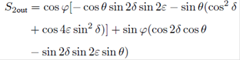
Examples of the trajectories we obtain for the evolution of an input linearly polarized signal propagating along an elliptically birefringent fiber with residual torsion are shown in Fig. 11. Again, the trajectories are not circular. In this case the curves are spherical trochoids whose amplitude depends on the azimuth angle of the input polarization state. In Fig. 11(a) we observe the trajectories depicted for five different azimuth angles of the input linear polarization (0, 20, 40, 60 and 80°) when the retardation δτ is larger than θ(δτ = 4.2θ). Consecutive loops have a different orbiting rate. They overlap only when δτ /θ is a rational number 17. In Fig. 11(b) the rotation angle θ is equal to the retardation angle of the elliptical retarder with residual torsion δτ .
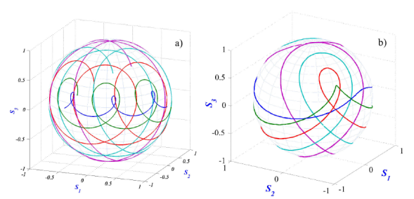
FIGURE 11 Trajectories of the polarization evolution of light along an elliptically birefringent fiber with residual torsion, represented on the Poincare´ sphere. a) δτ = 4.2θ (open curves). b) δτ = θ; these are closed curves (for retardations larger than 2π the next loop coincides with the previous one). In both figures the linearly polarized signals have different azimuth angles (0, 20, 40, 60 and 80 degrees). Trajectories are shown with: blue, green, red, light blue and purple lines, respectively
As we can see in Fig. 11, the symmetry of the curves related with the evolution of the polarization state does not allow the location of the polarization eigenmodes, nor the measurement of the ellipticity angle. Nevertheless, from Eq. (38) we can see that
In Fig. 12 we present the behavior of Stokes parameter S 3 for fibers with residual torsion and linear (Fig. 12(a)) or elliptical (Fig. 12(b)) retardation. These curves were calculated for different values of the azimuth angle of the input linear polarization φ(0, 30, 60, 90, 120 and 150°). When the retardation is linear, we can observe a symmetrical oscillation around the horizontal line for which S 3 is null. In this case ε = 0 and the curve associated to Eq. (39) overlaps with the horizontal line (S 3 = 0). For an elliptical retardation, the amplitude of the curve corresponding to φ = 0 is the lowest, and the minima are equal to zero.
5. Conclusions
Each one of the methods presented in this work can be used to determine some of the parameters that characterize the birefringence of single-mode optical fibers. But, to obtain a complete evaluation we must use a graphical method to measure the azimuth angle of the fast birefringence axis and the ellipticity angle of the fiber anisotropy, as well as a null polarimeter to measure the polarization beatlength.
In the presence of a residual torsion, analyzing the variation of Stokes parameter S3 it is possible to evaluate the ellipticity angle (allowing the identification of the type of retarder); while using a null polarimeter it is necessary to add a cold twist, varying the applied torsion until a periodic behavior of the polarization evolution is obtained. Under this condition, it is possible to measure the polarization beatlength and the ratio of the retardation angle to the total torsion angle.

