1. Introduction

Magnetic induction fields with a constant gradient play a key role in neutral atom traps ^1-3 and magnetic resonance imaging ^4-5, as discussed in our previous work on this topic ⁶. In particular, Ref. 4 reviewed the “Theory of Gradient Coil Design Methods for Magnetic Resonance Imaging”, recognizing that the search for the optimum coil windings is still open.

This Communication reports on a family of coil windings with Lamé spheroconal quadrupole harmonic distributions on spherical surfaces and their associated magnetic induction fields with constant gradients inside the spheres. The identification and construction of such a family is based on our succesive investigations on the rotations of asymmetric molecules, the Hydrogen atom, the harmonic oscillator, and the free particle ^7-11, leading to the identification of three families of ladder operators for the Lamé spheroconal harmonic polynomials ¹², and most recently to the formulation of the “Theory of Angular Momentum” in the bases of such harmonics ¹³.

The quadrupole spheroconal harmonics, with ℓ = 2, exist in five different species or parities under reflection in the respective cartesian coordinate planes: two of species ¹ or (+,+,+), and three of species xy, xz, and yz or (-,-,+), (-,+,-), (+,-,-), respectively. The last three are also spherical harmonics and were already included in Ref. 6, and consequently no more comments about them are made here. The other two familiar spherical harmonics, (2z ² - x ² - y ²)/2 and (x ² - y ²), are counterparts and special cases of the spheroconal harmonics of species ¹.

The main body of the article is written as follows: Section 2 identifies the scalar solutions of the Lamé differential equations, in which the Laplace equation separates in spheroconal coordinates. Section 3 constructs the vector magnetic potential inside, outside and continuous at the sphere. Section 4 leads to the magnetic induction field as the rotational of the potential inside and outside; its radial components are shown to be continuous at the spherical surface, while its transverse components are discontinuous giving a measure of the linear current density distribution; the lines of the latter are also evaluated in a closed form. Section 5 illustrates graphically the coil windings on the spherical surface, and the numerical coefficients for the cartesian components of the linear magnetic induction fields inside, with the respective discussions.

2. Lamé Spheroconal Quadrupole Harmonics of Positive Parities

The spheroconal harmonics are solutions of the Laplace equation, ∇2Φ=0, and common eigenfunctions of the square of the angular momentum operator, L ², and the asymmetry distribution Hamiltonian for the most asymmetric molecules, H*=(e1Lx2+e2Ly2+e3Lz2)/2. The three operators ∇ ², L ², and H* commute by pairs, and their respective equations are separable and integrable in spheroconal coordinates, x=r dnχ1|k12snχ2|k22, y=r cnχ1|k12cnχ2|k22, z=r snχ1|k12dnχ2|k22, involving Jacobi elliptical integral functions ^7,12,13-14. The quadratic dependence of the operators in the squares of the cartesian components of the angular momentum operator also guarantees that their eigenfunctions have well-defined parities under the reflection transformations x → -x, y → -y, z → -z.

Here, we concentrate on the quadrupole solutions with ℓ = 2 and positive parities (+,+,+). According with Table I in Ref. 12, the factorizable solutions

TABLE I Coefficients of cartesian components of internal magnetic induction field from Eq. (16), for sucessive values of the asymmetry distribution parameters σ [0,60 ], k12,k22, and the nodal elliptic cone numbers n₁ = 2, n ₂ = 0, and, n ₁ = 0, n₂ = 2, for the upper and lower signs, respectively. 

involve the common radial dependence of the familiar spherical harmonics, and the Lamé binomials:

(2)

in terms of the squares of the sn2χi|ki2 functions, with eccentricity parameters such that k12+k22=1, and

The separation constants have indices and eigenvalues such that:

and

counting the number of elliptical cone nodes in the eigenfunctions, and yielding the eigenvalue ℓ (ℓ + 1) of the square of the angular momentum, respectively.

Furthermore, the dynamic asymmetry distribution parameters in H* and the geometric parameters in the spheroconal coordinates are connected by k12=(e2-e3)/(e1\e3), k22=(e1\e2)/(e1\e3). The dynamic parameters are also connected by the conditions that their sum vanishes, and the sum of their squares is 3/2, so that only one of them can be chosen independently. They can also be written in terms of a single angular parameter 0 < σ < 60°: e1=cos(σ), e2=cos(σ-120∘), e3=cos(σ+120∘).

3. Vector Magnetic Potential Inside and Outside a Sphere

The vector magnetic potential is constructed by applying the operator generating infinitesimal rotations, r⃗×∇, to the Lamé spheroconal quadrupole harmonics identified in the previous section, guaranteeing that its divergence is zero. It is also required to be well-behaved inside and outside of a sphere of radius r = a, as well as continuous at the boundary. The radial part is common with the familiar Eqs. (4) and (5) in spherical coordinates ⁶, and the products of the Lamé binomials are the novelty elements:

(6)

(7)

Notice that there is no component in the radial direction, the orthogonality and right-handedness of the set of unit vectors r^, χ^1, χ^2 is taken into account, and the scale factors in χ1 and χ2 are the same ⁷:

The continuity condition at the boundary r = a is also satisfied.

4. Magnetic Induction Field Inside and Outside a Sphere

The magnetic induction field is evaluated via the rotational of the vector magnetic potential inside and outside the sphere:

(9)

The common angular operators including the scale factors in the radial terms of the magnetic induction fields, inside and outside the sphere,

are identified as the negative of the square of the angular momentum operator. Their eigenvalues are -2 × 3 when operating on Λn1(χ1)Λn2(χ2). On the other hand, taking into account the radial factor associated with each scale factor, as well as the radial derivatives of the radial functions in the transverse components, we recognize that B⃗ is proportional to r inside and inversely proportional to r ⁴ outside, describing its constant gradient and asymptotically vanishing behaviors in the respective regions.

Correspondingly, the radial components at the spherical boundary,

are continuous, consistently with Gauss’ Law. While the transverse components are discontinuous:

(11)

providing the linear density current distribution on the spherical surface according to Ampere’s Law.

The lines of the current distribution, dl⃗=χ^1hχ1dχ1+χ^2hχ2dχ2, are determined by the proportionality condition

This differential equation is exactly integrable leading to the closed form for the current distribution lines on the sphere of radius a:

passing by the point a,χ10,χ20.

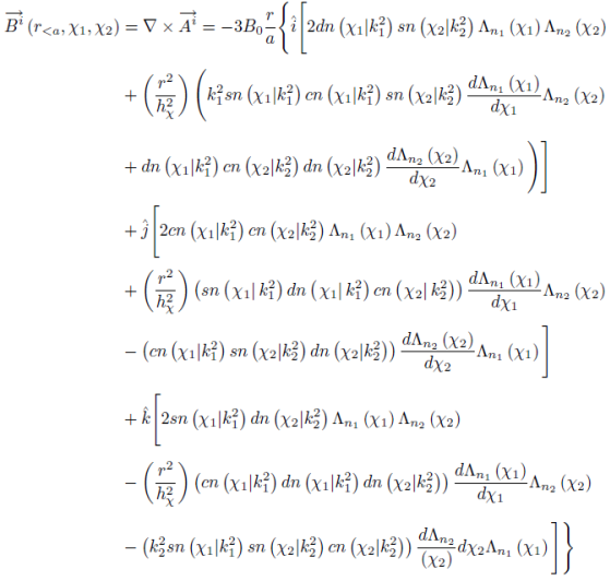
This section is completed by identifying the magnetic induction field inside the sphere in its cartesian coordinate representation. The task is started by replacing the unit vectors r^, χ^1, χ^2 in their cartesian components:

(14)

The arguments and parameters χi and ki2 are replaced by i = 1, 2 in the elliptical functions, simplifying the typography. The common angular denominator belongs to the square of the scale factor. The Lamé binomials are those of Eqs. (2), with derivatives:

Notice that we have chosen to separate the common factors of the magnetic induction field intensity and radial coordinate with the negative sign, and of the successive cartesian unit vectors. Notice also the common structure of the corresponding complementary factors differing in their specific spheroconal coordinate and spheroconal harmonic factors in each of the successive terms, to wit: the first terms with the common factors of 2 and the two Lamé binomials in the respective coordinates, associated with the original radial contributions; the angular terms with the common factor r2/hχ2, and involving the derivatives with respect to χ1 and χ2 of the respective Lamé binomial, respectively. Of the four terms in the product of the two Lamé binomials, only the first one with the value of one survives multiplying the common factor of 2; the other three -hn12(k12)sn2(χ1|k12)-hn22(k22)sn2(χ2|k22)+12hn12(k12)hn22(k22)sn2(χ1|k12)sn2(χ2|k22) cancel their counterparts from the angular terms. In fact, for the latter complementary factors involving the derivatives of the Lamé binomials also share the respective factors of the components of the unit radial vector along the cartesian directions, and in the remaining complementary factors, there are constant terms with the coefficients -hn12k12 and hn22k22, respectively, as well as terms in sn4χ1k12, sn4χ2k22, sn4χ1k12sn2χ2k22, and sn2χ1k12sn4χ2k22; each of the factors for the three cartesian directions turn out to be divisible byhχ2r2, with quotients that are respectively -hn22k22,0,-hn12k12, for the surviving terms, and terms in sn2χ1k12, sn2χ2k22, and sn2χ1k12sn2χ2k22 cancelling the radial contributions mentioned above. In conclusion, the cartesian composition of the magnetic induction field inside is:

(16)

The reader may ascertain that its divergence vanishes, taking into account Eqs. (4-5).

5. Graphical and Numerical Results and Discussion

In this section, the quadrupole spheroconal distributions of linear current densities on a spherical surface are illustrated in Fig. 1, and the coefficients for the associated interior magnetic induction fields in cartesian coordinates are reported in Table I, for different asymmetry distribution parameters and the two possible configurations of nodal elliptical cones, n ₁ = 2 and n ₂ = 0, respectively. Descriptions of the variations of the current distributions and magnetic induction fields, as the asymmetry distribution parameters and the nodal configurations change, as well as explanations and discussions about their relationships are given along the way.

FIGURE 1 Graphical illustrations of the quadrupole spheroconal harmonic windings on a spherical surface, Eq. (13), for the successive values of the asymmetry distribution parameter σ = 0, 5, . . . , 30−, 30+, . . . , 55, 60 degrees, and the nodal elliptical cone numbers n₁ = 2, n₂ = 0. 

The plotting of the lines on the spherical surfaces in Fig. 1 is based on Eqs. (13) and (1-5), using the asymmetry distribution parameters and their relationships described at the end of Sec. 2. The geometrical meaning of Eq. (13) corresponds to the line on the sphere passing through the point χ1=χ10,χ2=χ20 with a common value of the corresponding scalar spheroconal harmonic, from which the vector magnetic potential was constructed in Sec. 2. When using the spheroconal coordinates, introduced at the beginning of Sec. 1, it is important to distinguish the intervals of σ, [0,30) and (30, 60 ] with k12<k22 and k12>k22, for which the amplitudes of the respective variables cover the domains [0,2π], and [0,π], and [0,π], and [0,2π], respectively. In the specific case of the nodal ellitptic cone configuration with n ₁ = 2 and n ₂ = 0, in Fig. 1, the first and the final entries for σ = 0 and 60 correspond to the situations with rotational symmetry around the x-axis and z-axis, respectively, for which the corresponding spheroconal harmonics reduce to the familiar spherical harmonic counterparts Y ₂₂ (θ_x , φ_x ) with windings having components along both θ^x and φ^x and meridian circle separatrices, and Y ₂₀ (θ_z , φ_z ) with parallel circle windings and the equatorial circle as their separatrix, respectively. The reader may identify the correspondence of the corresponding windings with those in the figure of Ref. 6 at the top row of the middle column, and the two lower rows allowing for the change in orientations of their axes.

Next, we invite the reader to follow from the left to right the changes in the successive windings and their separatrices for σ =5, 10,…, 30^-, noticing the effects of the increasing distribution asymmetry. The value of σ =30 corresponds to the most asymmetric distribution, for which the domains and roles of the χ1 and χ2 variables are exchanged. Nevertheless the changes in the windings are continuous as illustrated by the windings in the middle of the figure above for σ =29, 30^-, and below 30⁺ and 31. The reader may now go on to follow the reduction of the blue winding area as the asymmetry distribution parameter σ increases up to 55^o and beyond.

The entries in Table I correspond to the asymmetry distribution parameters, σ, k12, and k22, and the coefficients in the cartesian representation of the interior magnetic induction field, for both nodal elliptical cone configurations, are obtained for Eqs. (13) and (3) with the explicit forms in the heading of the respective configurations. Notice that in each row in the Table, the values of k12 and k22 add up to one, as indicated in the paragraph of Eq. (2); also, the addition of the three coefficients is zero, reflecting the solenoidal nature of the magnetic induction field.

We describe first the systematic changes in the successive rows: the parameters σ and k12 share increasing values in their respective domains, accompanied by the consequently decreasing values of k22. All the coefficients in the x-component take decreasing values in the fourth column; and the coefficients in the z-component take increasing values in the sixth column, due to their respective k12 and k22, compositions. Notice, additionally, that the upper/lower entries for the pairs of σ and 60- σ, in the fourth and sixth columns are the same with the exchange between the x and z components. This is a consequence of the symmetries of the spheroconal coordinates, the spheroconal harmonics and their eigenvalues, under the exchanges of their variables χ1 and χ2 as discussed in ^7,13.

On the other hand, the reader may ask about the windings for the n ₁ = 0, and n ₂ = 2 configuration. Of course, they could also be calculated and plotted as already done for Fig. 1, but we prefer to invoke the symmetries recognized in the previous paragraph to formulate the answer. The shapes of the windings are the same as in Fig. 1, with the exchange of the numerical values of the parameters k12 and k22, the exchanges between x and z, and y self-converting, as suggested by the double entries in Table I. In other words, the counterpart of Fig. 1, for the other nodal configuration and the same values of σ and in the same order, starts from the windings of Y ₂₀(θ_x , φ_x ) with the x-axis of rotational symmetry, continues with those of its neighbors, passes through the most asymmetric distributions winding coinciding with that in Fig. 1, follows with those of the other neighors, approaching the final winding of the Y ₂₂(θ_z , φ_z ) with the z-axis of rotational symmetry. Shortly, the figure contains the same entries, with the shapes appearing in the reversed order and the x and z directions exchanged.

To conclude, this article presents the construction of the inner and outer vector magnetic potentials, Eqs. (6-7), from the application of the generator of rotations operator to the respective scalar spheroconal harmonic functions. The rotational operator acting on the magnetic vector potential leads to the respective magnetic induction fields, Eq. (9), with continuous radial components at the spherical boundary, Eq. (10), and with a discontinuity in their tangential components giving a measure of the linear current density distribution, Eq. (13). The field lines of the latter and their quadrupole spheroconal multipole nature are described analytically by Eq. (14) and illustrated in Fig. 1. Additionally, the cartesian coordinate representation of the target magnetic induction fields, with a constant gradient, is expressed analytically by Eq. (16) and examples of the numerical coefficients are contained in Table I. The illustrations and examples, restricted to the specifically chosen numercial values, can be easily extended for other choices.

The remaining step of this research is to find the representative loops of each winding providing the best approximations to the respective constant gradient magnetic inductions fields, and deviations from them, as counterparts of the Maxwell loops.

References

1. V. Gomer et al., Hyperfine Interactions 109 (1997) 281.
[ Links ]
2. http://nobel.prizes/physics/laureates/1997/
3. http://nobel.prizes/physics/laureates/2001/
4. S.S. Hidalgo-Tobon, Concepts in Magnetic Resonance 36 A (2010) 223.
5. http://nobel.prizes/medicine/laureates/2003/
6. L. Medina and E. Ley-Koo, Rev. Mex. Fis. E 57 (2011) 87.
7. E. Ley-Koo and R. Mendez-Fragoso, Rev. Mex. Fis. 54 (2008) 162.
8. E. Ley-Koo and A. Gongora, Int. J. Quantum Chem. 109 (2009) 790.
9. R. Mendez-Fragoso andE. Ley-Koo , Int. J. Quantum Chem. 110 (2010) 2765.
10. R. Mendez-Fragoso andE. Ley-Koo , Int. J. Quantum Chem. 111 (2011) 2882.
11. R. Mendez-Fragoso andE. Ley-Koo , Adv. Quantum Chem. 62 (2011) 137.
12. R. Mendez-Fragoso andE. Ley-Koo , Symmetry, Integrability and Geometry: Methods and Applications SIGMA 8 (2012) 74.
13. R. Mendez-Fragoso and E. Ley-Koo, Adv. Quantum Chem. 71 (2015) 115.
14. M. Abramowitz and I.A. Stegun, Handbook of Mathematical Functions with Formulas, Graphs, and Mathematical Tables, (Dover Publications, Inc., NY, 1965). pp. 569-574.
nueva página del texto (beta)
Inglés (pdf)
Artículo en XML
Referencias del artículo
Enviar artículo por email
Citado por SciELO