Implications of the Ornstein-Uhlenbeck-like fractional differential equation in cosmology

El-Nabulsi, Rami Ahmad; El-Nabulsi, Rami Ahmad

Servicios Personalizados

Revista

Articulo

Indicadores

Citado por SciELO
Accesos

Links relacionados

Similares en SciELO

Otros
Otros

Permalink

Revista mexicana de física

versión impresa ISSN 0035-001X

Rev. mex. fis. vol.62 no.3 México may./jun. 2016

Research

Implications of the Ornstein-Uhlenbeck-like fractional differential equation in cosmology

Rami Ahmad El-Nabulsi¹

^¹College of Mathematics and Information Science, Neijiang Normal University, Neijiang, Sichuan 641112, China. and Athens Institute for Education and Research, Athens, Greece, e-mail: nabulsiahmadrami@yahoo.fr

Abstract

In this paper we introduce a generalized fractional scale factor and a time-dependent Hubble parameter obeying an “Ornstein-Uhlenbeck-like fractional differential equation” which serves to describe the accelerated expansion of a non-singular universe with and without the presence of scalar fields. Some hidden cosmological features were captured and discussed consequently.

Keywords: FRW flat cosmology; generalized fractional scale factor; Ornstein-Uhlenbeck-like fractional differential equation; Mittag-Leffler function; Gauss-Bonnet invariant

PACS: 98.80Jk; 02.30.Gp

1.Introduccion

In recent years, increasing attention has been focused on the applications of fractional differential and integral operators to different branches of applied sciences and it has contributed a lot to mathematical physics and theoretical physics ¹^,²^,³. In fact, the use of fractional calculus in many fundamental physical problems has attracted theorists to pay more attention to accessible fractional calculus tools that can be used in solving numerous problems of theoretical physics and quantum field theories ⁴^-¹⁵. Recently, it was observed that fractional calculus plays an interesting role as well in cosmology and the physics of the early universe where some hidden properties are captured and analyzed in details (¹⁶^,¹⁷^,¹⁸ and references therein). In a more recent work, we have we have discussed the Friedman-Robertson-Walker (FRW) cosmology characterized by a scale factor obeying different independent types of fractional differential equations with solutions given in terms of and generalized Kilbas-Saigo-Mittag-Leffler functions ¹⁹. It was observed that this new fractional cosmological scenario exhibits some interesting results like the occurrence of an accelerated expansion of the universe dominated by the dark energy (DE) and the occurrence of a repulsive gravity in the early stage of the universe and time-decaying cosmological constant without the presence of scalar fields. In this paper, we would like to generalize this approach by introducing a new generalized fractional form of the scale factor in terms of the Hubble parameter and discuss its implications in the absence and in the presence of scalar fields. Our basic motivation to deal with a generalized fractional scale factor (GFSF) is based on the fact that the Hubble parameter which describes the expansion of the universe is considered one of the most important parameter in cosmology as it is used to estimate the age and the size of our universe. Considerable progress has been made in determining the Hubble constant and deducing its time-dependence since theories and observations predict that the Hubble parameter varies with time ²⁰^,²¹. Although there exist in literature a large number of phenomenological theories to describe the accelerated expansion of the universe ²²^-³⁰, we consider that using fractional differential operators to describe cosmological scenarios is of considerable interest since fractional-order derivatives and integrals are nonlocal operators and hence one expects them to play important roles in cosmology ³¹^,³². Therefore, one expects more hidden properties are present in cosmology with a GFSF that deserve to be captured and analyzed.

The paper is organized as follows: in Sec. 2, we introduce the main definitions and setups for the case of a FRW flat cosmology with a GFSF and a time-dependent Hubble parameter and we discuss some features in the absence of the scalar field whereas the presence of the scalar field will be discussed in Sec. 3; we consider the case of a cosmology with a Gauss-Bonnet gravity for reasons that will be mentioned in the same section; finally conclusions and perspectives are given in Sec. 4.

2. FRW cosmology with a generalized fractional scale factor

By using the following FRW metric for a flat universe ds2=-dt2+a2(t)(dr2+r2(dθ2+sin2θdϕ)) where α(t) is the scale factor, the Hubble parameter is defined usually by H(t)=ȧ(t)/a(t) and accordingly for the case of a constant Hubble parameter, e.g.H=H0, it is easy to check using da=aH(t)dt that the scale factor is obtained from the integral equation a(t)-a0=H0∫0ta(u)du. However, there are some arguments that show that the Hubble parameter is related to the scale factor ³³^,³⁴^,³⁵^,³⁶. In this paper, we will conjecture that the Hubble parameter varies as H(t)=ηH0+σF(t)/a where ƞ and σ are real constants and F(t) is a time-dependent function. In that case, we have da=a(t)H(t)dt=a(t)(ηH0+σF(t)/a(t))dt=ηH0a(t)dt+σF(t)dt and therefore ȧ(t)=ηH0a(t)+σF(t). This equation is similar to the Ornstein-Uhlenbeck stochastic differential equation ³⁷. The fractional version of this differential equation may be written as: 0Dtαa(t)=ηH0αa(t)+σF(t) where 0Dtαa(t)=(1/Γ(α))∫0t(t-τ)α-1a(τ)dτ is the Riemann-Liouville fractional integral (RLFI) with 0Dtαa(t)=a(t). We entitled this equation the “Ornstein-Uhlenbeck-like fractional differential equation” (OULFDE). Here 0<α<1 is the fractional exponent. Applying the fractional integral operator to both LHS and RHS of 0Dtαa(t)=ηH0αa(t)+σ(t) we can find the solution of the OULFDE which is given by ³⁷:

a(t)=a0E1,α(ηH0αtα)+σ∫0tF(τ)(t-τ)α-1Eα,α(ηH0α(t-τ)α)dτ, 1

where

Eα,β(z)=∑k=0∞zkΓ(α+βk)

is the Mittag-Leffler function ³⁸.

2.1

We choose at the beginning F(t)=F0tλ-1 where F ₀ is a real parameter and λ is a real constant. Using the fact that³⁹:

∫0tτλ-1(t-τ)α-1Eα,α(ηH0α(t-τ)α)dτ=Γ(λ)tα+λ-1Eα,α+λ(ηH0αtα), 2

we can write the solution (1) as:

a(t)=a0E1,α(ηH0αtα)+σF0Γ(λ)tα+λ-1Eα,α+λ(ηH0αtα). 3

We can set for simplicity a0=η=H0α=σ=F0=1 and then Eq. (3) is simplified to:

a(t)=E1,α(tα)+Γ(λ)tα+λ-1Eα,α+λ(tα)=∑k=0∞tkαΓ(α+k)+Γ(λ)tα+λ-1∑k=0∞tkαΓ(α+(α+λ)k),=1Γ(α)+tαΓ(α+1)+t2αΓ(α+2)+…+Γ(α+2)tα+λ-1(1Γ(α)+tαΓ(2α+λ)+t2αΓ(3α+2λ)+…)=1Γ(α)(1+Γ(λ)tα+λ-1)+(1Γ(α+1)+Γ(λ)tα+λ-1Γ(2α+λ))tα+(1Γ(α+2)+Γ(λ)tα+λ-1Γ(3α+2λ))t2α+… 4

One particular choice of parameter is obtained if for instance we set λ=1-α which reduces Eq. (4) to:

a(t)=1+Γ(1+α)×(1Γ(α)+1Γ(α+1)tα+1Γ(α+2)t2α+…)≡1+Γ(1+α)E1,α(tα), 5

and therefore the scale factor is increasing with time and a universe dominated by such a form of a scale factor is accelerated with time and is non-singular. In conclusion, Eq. (5) is the solution of the fractional differential equation 0Dtαa(t)=a(t)+t-α and the Hubble parameter varies as H(t)=ηH0+σF(t)/a=1+t-α/a or more explicitly as:

H(t)=1+1tα(1+Γ(1-α)(1Γ(α)+1Γ(α+1)tα+1Γ(α+2)t2α+…))≡1+1tα(1+Γ(1-α)E1,α(tα)). 6

In our model the Einstein’s field equations that govern our model of consideration are Rμν-gμνR/2+Λgμν=8πGTμν, Λ is the cosmological constant, G is the gravitational coupling constant assumed both to be time-dependent and Tμν=(p+ρ)uμuν+pgμν the stress-energy momentum tensor. p and p are respectively the pressure and density of the perfect fluid and uμ is the fluid rest-frame four velocity. The field equations give the following Friedmann equation ȧ2/a2=8πGρ/3+Λ/3 and the conservation equation for the stress energy-momentum tensor i.e. T:νμν=0 gives Λ̇+8πĠρ+8πG(ρ̇+3ȧ(ρ+p)/a)=0 ⁴⁰. For complete determinacy of the system, we will adopt the equation of state (EoS) p=ω(t)ρ where ω is the EoS parameter assumed to be time-dependent. It is believed that the universe is presently in a stage of an accelerated expansion (dark energy dominance) and decelerated expansion in the past (dark matter dominance). Therefore, one naturally expects that the EoS parameter varies with time ⁴¹^,⁴². In our model, we assumed that both and vary with time. This choice is not new and it was considered in a large number of cosmological scenarios In fact, a time-dependent lambda is favored as a constant fails to explain the enormous difference between the cosmological constant inferred from observation and the vacuum energy density obtained from quantum field theories. Besides, a time-dependent gravitational constant has many interesting cosmological and astrophysical consequences (see ⁴³ and references therein). we can now split the equation Λ̇+8πĠρ+8πG(ρ̇+3ȧ(ρ+p)/a)=0 into two independent equations: Λ̇+8πĠρ=0 and ρ̇+3ȧ(ρ+p)/a=0. In order to solve the previous cosmological equations, we conjecture that the cosmological constant varies as Λ(t)=3χȧ2/a2 where χ is a real parameter. Such an ansatz was considered by many authors and has many interesting cosmological consequences ⁴⁸^,⁴⁹^,⁵⁰. Using the relations

ddxEα,β(x)=1αx(Eα,β(x)-(β-1)Eα,β(x))

and

limx→∞Eα,β-1(x)/Eα,β(x)≈1

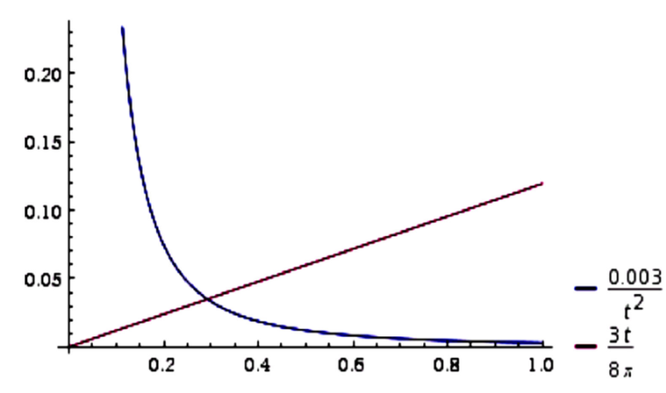
⁵¹, the cosmological constant varies as:

Λ(t)=3χ(1tαE1,α-1(tα)-(α-1)E1,α(tα)1+Γ(1-α)E1,α(tα))t→+∞2≈3χ(1tα(2-α)E1,α-1(tα)1+Γ(1-α)E1,α(tα))2≈3χ((2-α)Γ(1-α))21t2α 7

Accordingly the Friedmann equation gives:

8πGρ3≈(1-χ)1tα(2-α)Γ(1-α)2 8

The differential equation Λ̇+8πĠρ=0 gives now: 8πĠρ=6χα(2-α)2t-2α-1/Γ2(1-α) and therefore using Eq. (8) we find Ġ/G=2χα/(1-χ)t or after simple integration G=kt2χα/(1-χ) where k is a constant of integration. Therefore the energy density decays as

ρ=3(1-χ)8πk(2-α)Γ(1-α)2t-2α/(1-χ), 9

with χ<1 in order to obtain a positive energy density. The continuity equation ρ̇+3ȧ(ρ+p)/a=0 with p=ω(t)ρ gives now the following time-dependent EoS parameter:

ω(t)≈-1+2α3(1-χ)×1t+t1-α1+Γ(1-α)E1,α(tα)t→+∞≈-1+2α3(1-χ)1t. 10

For 0<α<1, the EoS parameter decreases with time and tends asymptotically toward ω = 1. Hence the universe in such a scenario is non-singular, accelerating with time and is dominated for very large time by a vacuum energy. The cosmological constant decays in time, the gravitational constant increases with time for 0<χ<1. We plot in Figs. 1-4 the variations of the EoS parameter, the gravitational constant, the scale factor and the cosmological constant for χ=1/2 and different values of α.

Figure 1 Variations of ω(t) for α = 1=4; 1=3; 1=2; 2=3.

Figure 2 Variations of G(t) for α = 1=4; 1=3; 1=2; 2=3.

Figure 3 Variations of α(t) for α = 1=2; 2=3 up to the 1st four orders.

Figure 4 Variations of Λ(t) for α = 1=4; 1=3; 1=2; 2=3

For α≥2/3, the scale factor increases acceleratedly with time than the rest values of α. We can estimate the relative variation of the gravitational constant Ġ/G=2χαt-1/(1-χ). For χ=1/10, we find Ġ/G=2α/t. For χ=103, we find a small relative variation Ġ/G=0.002α/t and therefore for 0<α<1, we find a relatively small Ġ/G, e.g. for α =1/2, we find Ġ/G=103/t and therefore the present day variation of the gravitational constant is Ġ0/G0=0.001/t0≈10-13yr-1 which is in agreement with recent observations ⁵²^,⁵³. Here t₀ is the present age of the universe.

2.2

We can choose F(t)=F0tλ-1Eα,λ(-tα). Using the fact that ³⁷:

∫0tτλ-1Eα,λ(-τα)(t-τ)α-1Eα,α((t-τ)α)dτ=tα+λ-1E2α,α+λ(t2α), 11

then from Eq. (1) the scale factor evolves as:

a(t)=E1,α(tα)+tα+λ-1E2α,α+λ(t2α). 12

For λ = 1 -α, Eq. (12) is reduced to: a(t)=E1,α(tα)+E2α,1(t2α)≈E2α,1(t2α). Using

Eα,β(z)=∑k=0∞zkΓ(α+βk),

we can write:

a(t)≈E2α,1(t2α)=1Γ(2α)+t2αΓ(2α+1)+t4αΓ(2α+2) 13

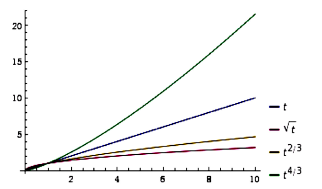
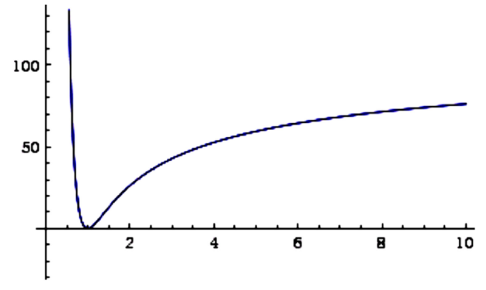
The scale factor in that case increases faster than in the previous case and the universe is non-singular. To illustrate graphically, we plot in Fig. 5 the variations of the scale factor for both cases F(t)=F0tλ-1Eα,λ(-tα) and F(t)=F0tλ-1 mainly for α = 1/2.

Figure 5 Variations of α(t) for Ft=Fotλ-1Eα,λ(-tα) (blue line) and Ft=Fotλ-1 (red line) mainly for α = 1/2.

For Λ(t)=3χȧ2/a2, we find

Λ(t)=(3χ/4α2t4α)( Eα.0(t2α)/ E2α.1(t2α))2≈3χ/4α2t4α∝t-4α

whereas for F(t)=F0tλ-1 we find Λ(t)∝t-2α and therefore the cosmological constant in that cases decays more rapidly than in the previous case as show in Fig. 6. It is easy to check that in that case the energy density decays with time as ρ(t)∝t-4α/(1-χ) whereas in the previous case we found ρ(t)∝t-2α/(1-χ) and that the EoS parameter decays as ω(t)≈-1+4α/3(1-χ)t. In that case as well, the gravitational constant increases with time as G=kt4χα/(1-χ) with 0<χ<1. The universe is therefore asymptotically dominated by a cosmological constant. In summary, the phenomenological law H(t)=ηH0+σF(t)/a and the OULFDE 0Dtαa(t)=ηH0αa(t)+σF(t) reveal new interesting properties not found in the standard FRW model mainly the occurrence of a non-singular universe and its accelerated expansion with time. For F(t)=F0tλ-1Eα,λ(-tα), the universe is accelerated more speedily than for F(t)=F0tλ-1 and is dominated for vary large time by a vacuum energy. One may argue that for

F(t)=F0tλ-1Eα,λ(-tα)E2α,λ(-t2α)E3α,λ(-t3α)…Enα,λ(-tnα)≡F0tλ-1Πi=1nEiα,λ(-tiα),

we find a(t)≈tα+λ-1Enα.nα+λ(tnα) and accordingly the universe expands vary rapidly with time and the cosmological constant decays speedily with time and is non-singular. It is notable to note that for α = 1, the scale factor exhibits an exponentially behavior which corresponds for inflation or superinflation depending on the form of F(t) since the Mittag-Leffler function reduces to the exponential function.

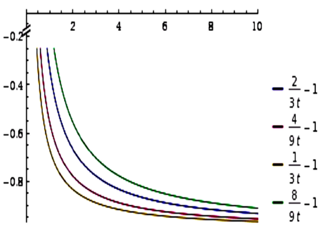
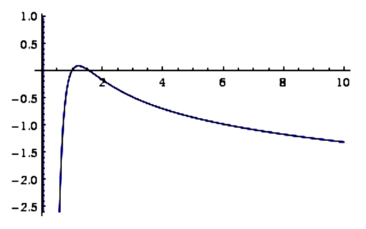
Figure 6 Variations of Λ(t) for Ft=Fotλ-1Eα,λ(-tα) (blue line) and Fotλ-1 (red line) mainly for α = 1/2.

It is noteworthy that for α = 1 and for σ = 0, i.e. absence of F(t) , the fractional differential equation 0Dtαa(t)=ηH0αa(t)+σF(t) is reduced to 0Dtαa(t)=ηH01a(t) which is nothing than the definition of the Hubble parameter. In that case, Eq. (3) which gives the evolution of the scale factor with time is reduced accordingly to a(t)=a0E1.1 which is an exponential growth and corresponds to an inflationary scenario. This proves that our basic solutions which are represented merely by Eqs. (9), (10) and (13) are due to the use of the new mathematical tool. These solutions are interesting otherwise the model gives rise to internal inflation which is not favored in cosmology.

3. FRW cosmology with a generalized fractional scale factor and with a scalar field

Despite that the OULFDE offers the standard FRW model many desirable features in the absence of scalar fields it will be of interest to know the effects of OULFDE on the FRW model with single scalar field. It is believed that scalar fields can account for both an accelerated exponentially expansion of the early universe as well for the late-time accelerated expansion of the universe ⁵⁴^,⁵⁵. However, there are recent approaches which suggest that a non-minimally coupled field to the scalar curvature can generate dark energy and even dark matter ⁵⁶. It is notable that the coupling of the scalar field to curvature appears in alternative theories of gravities which could be responsible after compactification of higher dimensions for the current accelerated expansion. Some nice alternatives theories include the string-inspired dilaton gravities, Kaluza-Klein theory, M/string theory and higher derivative theories with correction terms of higher-orders in the curvature ⁵⁷^,⁵⁸. These correction terms may play a significant role in the inflationary epoch. The leading quadratic correction terms correspond to the Gauss-Bonnet (GB) curvature invariant which appears in the tree-level effective action of the heterotic string ⁵⁹^,⁶⁰. In four-dimension, the GB term is a topological invariant, ghost-free in Minkowski background, its appearance alone in the action can be neglected as a total divergence. However, if coupled, it affects the cosmological dynamics in presence of dynamically evolving dilaton and modulus fields at the one-loop level of string effective action and may have desirable features in many cosmological scenarios, e.g. avoiding the initial singularity of the universe ⁶¹. Many of inflationary potentials are disfavored when constrained to Planck CMB data due mainly to the large tensor-to-scalar ratio yet it was argued in ⁶² that non-minimal coupling to the GB term may set these potentials in good agreement with the Planck data. There are many research papers discussing the scalar field cosmology with GB curvature corrections as possible solutions to DE with a field-dependent scalar potential ⁶³^-⁶⁶. In this section, we investigate a cosmological FRW model in which a single dynamical scalar field is minimally coupled to gravity in the presence of the GB invariant and a scale factor governed by the OULFDE. However, in this section we assume that G is constant and we set 8πG=c=h=1. The action of the theory is:

S=∫-gd4x(R2-12∂μϕ∂μϕ-V(ϕ)+f(ϕ)G)+Smatter, 14

where g is the metric, V(ϕ) is the scalar potential assumed here to be flat and of the form V(ϕ)=Λ, Λ is a real parameter, G=R2-4RμνRμν+RμνρσRμνρσ is the GB invariant, f(ϕ) is a coupling function which works as the effective potential for the inflaton field and Smatter=∫-gd4xLmatter is the action for ordinary matter with La grangian L _matter for perfect fluid with density ρ and pressure p. In fact, a flat potential i.e., a cosmological constant is consistent with the field moving along an almost flat potential like a pseudo-Goldstone boson and is in agreement with observations ⁶⁷. Therefore one expects that Λ≪1. The resulting field equation is obtained after varying the total action with respect to the metric:

Rμν-12gμνR-12(∂μϕ∂νϕ-12gμν∂ρϕ∂ρϕ)-12gμν(-V(ϕ)+f(ϕ)G)-2(∇μ∇νf(ϕ))R+2f(ϕ)(RRμν-2RσμRνρ+RμρστRρστν-2RμρσνRρσ)+4(∇ρ∇μf(ϕ))Rνρ+4(∇ρ∇νf(ϕ))Rνρ+2gμν(∇2f(ϕ))R-4(∇2f(ϕ))Rμν-4gμν(∇ρ∇σf(ϕ))Rρσ+4(∇ρ∇σf(ϕ))Rμρνσ=Tμν. 15

gμν is the metric tensor components, ∇ν is the contra-covariant derivative and Tμν is the usual stress energy-momentum tensor. Considering the spatially-flat Friedmann-Robertson-Walker (FRW) metric, the dynamical equations are given by ⁶⁸:

12ϕ̇2-3H2+V(ϕ)-24ϕ̇dfdϕH3+ρ=0, 16

-2H˙+3H˙2=12ϕ˙2-V(ϕ)+8H2ϕ¨dfdϕ+8Hϕ˙2d2fdϕ2+16HH˙ϕ˙dfdϕ+16H3ϕ˙dfdϕ+p. 17

By varying the action over the scalar field, we obtain:

ϕ̈+3Hϕ̇+dVdϕ-24dfdϕ(ḢH2+H2)=0. 18

In addition, the continuity equation for the present model ρ̇+3H(p+ρ)=0 is still satisfied. In this section, we choose F(t)=F0tλ-1Eα,λ(-tα) which gives the following evolution of the scale factor a(t)≈E2α,1(t2α) and consequently the time-dependent Hubble parameter H(t)=(1/2αt2α)(E2α,0(t2α)/E2α,1(t2α))≈(1/2αt2α). Besides, we assume that the coupling function varies as f(ϕ)=f0ϕε where f0 is a real parameter set equal to unity for simplicity and ɛ is a real constant ⁶⁹. From Eq. (18), the following 2^nd-order differential equation holds accordingly:

ϕ̈+32αt2αϕ̇-6εϕε-1α2t6α14α2t2α-1t=0. 19

The dynamics depends accordingly on the value of the fractional parameter α. We discuss the following two independent cases:

3.1

For α = 1/2, the following 2^nd-order linear differential equation for the scalar field ϕ̈+3ϕ̇/t=0 holds ∀ε and the solution is given by ϕ(t)=c2+c1t-2 where c ₁ and c ₂ are integration constants. For illustration purpose, we can set ϕ(1)=0 and ϕ̇(1)=1 which gives the following evolution for the scalar field ϕ(t)=(1-t-2)/2 and accordingly, the energy density behaves as:

ρ(t)=3t2-1t3-Λ+24ε1t6ϕε-1, 20

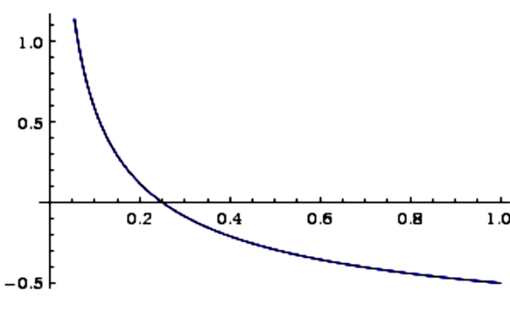
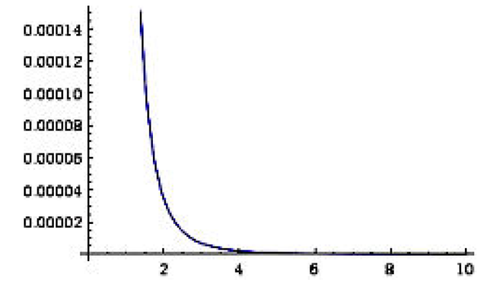
We plot in Fig. 7 the variations of the energy density with time for ɛ = 1 and ɛ = 2 assuming Λ≈0 and in Fig. 8 the variations of the scalar field with time:

Figure 7 Variations of p(t) for ɛ = 1 and ɛ = 2.

Figure 7 shows that for ɛ = 2 the energy density was negative at the early stage of the evolution. A negative energy density in the early universe was discussed recently in⁷⁰ and has many physical impacts on inflationary epoch. For ɛ = 1 the continuity equation ρ̇+3H(p+ρ)=0 with p=ω(t)ρ gives the following time-dependent EoS parameter:

ω(t)=-1+2t-3-t-4+48t-73t-3-t-4+24t-7. 21

For ɛ = 2, we find

ω(t)=-1+2t-3-t-4+48t-7-96t-133t-3-t-4+24t-7-24t-13. 22

Their variations with time are plotted in Figs. 9 and 10.

Figure 8 Variations of ϕ(t).

Figure 9 Variations of ω(t) for ɛ = 1.

Figure 10 Variations of ω(t) for ɛ = 2.

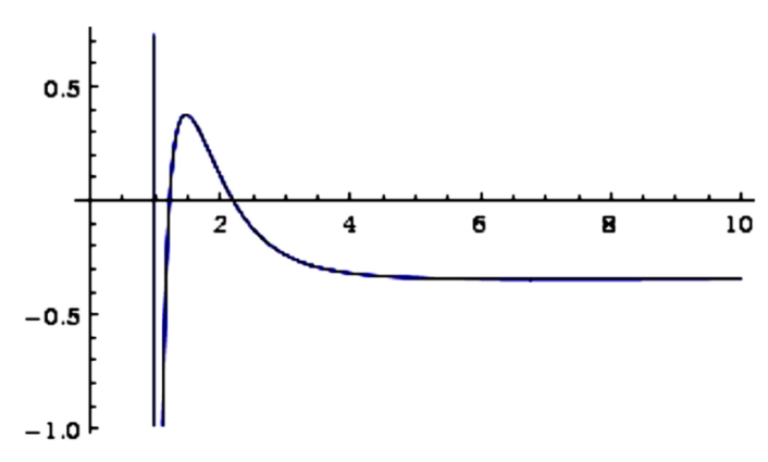
For ɛ = 1 the EoS parameter decreases with time and tends toward a stable value close to -0.335 which is within the range of observational limits ⁷¹^,⁷² whereas for ɛ = 2, the EoS parameter decreases from a larger positive value toward a negative stable value close as well to -0.335. This case shows that the early universe is not necessarily dominated by a negative pressure matter with a positive energy density. The behavior of the EoS parameter shows that for ɛ = 1 and ɛ = 2 the phantom-divide line is not crossed in our scenario.

3.2

For α = 1/4 and ɛ = 1, the following 2^nd-order linear differential equation for the scalar field

ϕ̈+6t1/2ϕ̇-96t3/24t1/2-1t=0, 23

and the solution is given by:

ϕ(t)=c3e-12tt+112-128t+c4, 24

where c3 and c4 are integration constants. We set for numerical illustrations ϕ(1)=0 and ϕ̇(1)=1 which reduces Eq. (24) to:

ϕ(t)=18e12-12t(84t+7)-1024t+933, 25

Accordingly, the energy density varies as:

ρ(t)=12t-1+192(64t-3/2-63e12-12t)t-3/2-12(64t-3/2-63e12-12t)2-Λ. 26

Accordingly, the EoS parameter varies asymptotically as

ω(t)≈-1+t-2+2560t-46t-3/2+5120t-7/2. 27

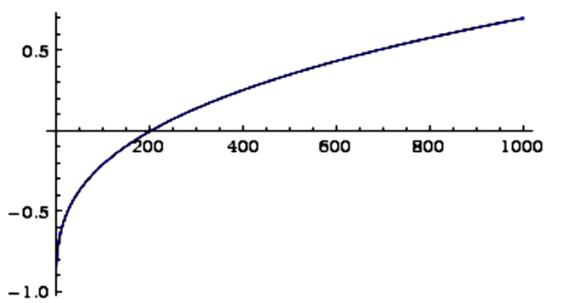
We plot in Figs. 11-13 respectively the variations of the scalar field, the energy density and the EoS parameter with time:

Figure 11 Variations of ϕ(t) for ɛ = 1 and α = 1=4.

Figure 12 Variations of p(t) for ɛ = 1 and α = 1=4.

Figure 13 Variations of ω(t) for ɛ = 1 and α = 1=4.

In that case the EoS parameter tends asymptotically toward ω = -1 at the present epoch. The universe in non-singular, expanding acceleratedly with time and is dominated by a cosmological constant at very late time. The energy density was negative in the past, increases toward a positive value then decreases toward zero with time. The expansion of the early universe is due to the negative energy density with the negative pressure and the late-time accelerated expansion comes from the positive energy and the negative pressure which behave like a dark energy. It is amazing that the non-singular universe is expanding with time whereas a transition from a negative energy density to a positive energy density occurs during its dynamical evolution. Similar scenario occurs in ⁷³ and negative energies density in accelerated universe was discussed recently in ⁷⁴.

Let us at the end mention that for the case of a time-dependent gravitational constant and cosmological constant with Λ(t)=3χȧ2/a2 and a general a nearly flat potential v(ϕ)≪1, we find Λ(t)≈3χ/4α2t4α as obtained in the previous section whereas Eq. (16) takes now the general form:

12ϕ̇2-3H28πG+V(ϕ)-24ϕ̇dfdϕH3+ρ+Λ8πG=0, 28

and accordingly, we find after simple algebra assuming α=1/2 and ε=1i.e. ϕ(t)=(1-t-2)/2

ρ(t)≈3(1-χ)8πGt2-1t3+24t6. 29

Assuming χ≪1 then the differential equation Λ̇+8πĠρ=0 then gives asymptotically after simple algebra G(t)≈3t/8π which shows that the gravitational coupling constant increases linearly with time and therefore the energy density is positive and decays as ρ(t)≈2/t3+24/t6.

Accordingly, the EoS parameter decays as ω(t)=-1+(t-4+24t-7/(t-4+12t-7) and asymptotically it tends toward 0 which corresponds for a pressureless matter. The non-singular universe is then accelerating with time, its energy density is positive and decays with time, the gravitational constant increases with time whereas the cosmological constant decays in time and there is no place to dark energy in such a scenario. Accelerated expansion of the universe free from a dark energy component is discussed recently in ⁷² based on thermodynamical frameworks. Figures 14 and 15 illustrate respectively the variations of ω(t) versus p(t) and the variations of Λ(t) versus G(t) with time:

Figure 14 Variations of ω(t) versus p(t).

Figure 15 Variations of Λ(t) versus G(t).

The present time relative variation of the linearly increasing gravitational constant is Ġ0/G0=H0 which is also within the range of observations.

For α = 2/3 and ɛ = 1, we find Λ(t)≈9χ/16t8/3 and from Eq. (19), we get:

ϕ̈+94t4/3ϕ̇-272t4916t4/3-1t=0, 30

and the solution is given by:

ϕ(t)=c5(Ei(272t3)+e274t3(278t23+t+72932t3))-98t3+c6, 31

where c₅ and c₆ are constants of integration; Ei(x) is the exponential integral. To illustrate numerically, we set ϕ(1)=0 and ϕ̇(1)=1 which reduces Eq. (31) to:

ϕ(t)=373977e34Ei272t3-Ei274t3-76e341+9t332t23+108t3+729t103+4e15216799t3-2881024e152t3 . 32

Asymptotically, at t=∞, we can approximate Eq. (32) by ϕ(t)≈-19te-27/4/8 and therefore the energy density varies as

ρ(t)≈27(1-χ)16t8/38πG-1539e-27/464t4 . 33

Assuming χ≪1 then we obtain from the differential equation Λ̇+8πĠρ=0 for very large time G(t)≈2.4t4/3 which corresponds for an increasing gravitational constant and therefore the energy density is positive and decays as ρ(t)≈0.000056t-4. Hence, the EoS parameter decays as ω(t)≈-1+0.17t1/3 which increases slowly in time. The non-singular universe is accelerating with time, its energy density is positive and decays with time, the gravitational constant increases with time whereas the cosmological constant decays in time and the EoS parameter increases from -1 toward a positive value asymptotically. We plot in Figs. 15-18 the variations of.

Figure 16 Variations of ϕ(t) represented by Eq. (32).

Figure 17 Variations of Λ(t) versus G(t).

Figure 18 Variations of p(t) with time.

Figure 19 Variations of ω(t) with time.

We left other values of for interested readers.

It is notable that for α = 1 and σ = 0, the scale factor a(t)≈E21,1(t2) which corresponds for a super-inflationary regime. The dynamics of the scalar field is obtained from Eq. (19) which will be reduced to

ϕ̈+32t2ϕ̇-6εϕε-1t61t2-1t=0 . 34

The dynamics therefore differs from previous solutions obtained for α ≠1. For example, for ɛ = 1, the solution is given by:

ϕ(t)=-32c7Ei(32t)+c8te32t+c9+1t5(189.63t6+284.4444t5log⁡t-213.333t4-53.333t3-13.333t2-3t-0.8), 35

which differs completely from previous solutions obtained. c₇,…,c₉ are constants of integration The solution depends on initial conditions and is constrained by t>0. This also proves that our solutions are due to the use of the new mathematical tool and give rise to more generalized solutions and cosmological features.

4. Conclusions and Perspectives

In this paper, we have tried to show that fractional calculus plays an important role in modern cosmology and a number of properties were hidden and deserve to be captured. Through this paper, we have considered a GFSF which obeys the OULFDE with a particular Hubble parameter of the form H(t)=ηH0+σF(t)/a. Such a particular form of the Hubble parameter allows the scale factor of the universe to satisfy a differential equation similar to the Ornstein-Uhlenbeck stochastic differential equation. In this work, we have considered the fractional version of this equation which is the OULFDE which gives already a non-singular acceleratedly expanding universe due to the mathematical properties of the Mittag-Leffler function obtained in the corresponding solution. We have considered the flat FRW model in the absence and in the presence of a scalar field.

In the absence of the scalar field and for the case of a flat FRW model with time-dependent gravitational constant and a time-dependent cosmological constant varying as Λ(t)=3χȧ2/a2, it was observed that for F(t)=F0tλ-1 ×Eα,λ(-tα) and for α = 1/2, the non-singular universe is dominated by a decaying cosmological constant, a decaying positive energy density and the gravitational constant increases with time 0<χ<1. The universe is therefore asymptotically dominated by a cosmological constant. It is interesting to obtain such interesting properties without the presence of scalar fields and higher-order corrections terms or even modifying the gravity theory. For χ≪1, the cosmological constant is too small and the present day variation of the gravitational constant is relatively small and within the range of observations.

In the presence of the scalar field and higher-order GB curvature term, the dynamical equations offer some new features. For the case of a constant and Λ, the dynamics depend on the form of the GB coupling function f(ϕ)∝ϕε. For ɛ = 1 and α = 1/2 the EoS parameter decreases with time and tends asymptotically toward -0.335 whereas for ɛ =2, the EoS parameter was positive at early time then decreases toward -0.335. This special feature signifies that the early universe is not essentially dominated by a negative pressure matter with a positive energy density. For α = 1/4, the EoS parameter tends asymptotically to ω = 1. The energy density of the universe was negative in the early epoch, then a transition from a negative value to a positive value occurs and finally it decreases toward zero at late time. However, in the presence of time-dependents G and Λ, it was observed that for α = 1/2, the non-singular acceleratedly expanding universe is dominated by a positive energy density which decays with time, a linearly increasing gravitational constant, a decaying cosmological constant and an EoS parameter which tends to zero at very large time. This scenario is free from the presence of the DE component. For α = 2/3 and ɛ = 1, the non-singular acceleratedly expanding universe is dominated by a decaying positive energy density with time, an increasing gravitational constant and a decaying cosmological constant whereas the EoS parameter increases from -1 toward a positive value asymptotically.

These features prove that fractional calculus deserves to be considered seriously in cosmology and physics of the early universe. Both the GFSF and the OULFDE offers new insights in modern cosmology and it will be of interest to explore in details in the future their impacts on the dark energy problem and the quantum physics of the universe. It will be interesting to explore in the upcoming work whether the present fractional model may be tested by future observational data fittings.

Acknowledgments

I would like to thank the anonymous referees for their useful comments and valuable suggestions.

References

1. R. Herrmann, Fractional Calculus: An Introduction for Physicist, World Scientific, River Edge, New Jersey, 2nd edition, (2014). [ Links ]

2. R. Hilfer, Applications of Fractional Calculus in Physics, (Ed.) World Scientific, Singapore, (2000). [ Links ]

3. J. Sabatier, O.P. Agrawal, J.A. Tenreiro Machado, Theoretical Developments and Applications in Physics and Engineering, (Eds.) Advances in Fractional Calculus. Springer, Dordrecht, (2007). [ Links ]

4. R. Herrmann, Physica A 389 (2010) 693. [ Links ]

5. R. Herrmann, Physica A 389 (2010) 4613. [ Links ]

6. R. Herrmann, Int. J. Mod. Phys. B 27 (2013) 1350019. [ Links ]

7. R. Herrmann, Cent. Europ. J. Phys. 11 (2006) 1212. [ Links ]

8. E. Goldfain, Chaos, Solitons Fractals 28 (2006) 913. [ Links ]

9. E. Goldfain, Comm. Nonlin. Sci. Num. Simul. 13 (2008) 1397. [ Links ]

10. E. Goldfain, Comm. Nonlin. Dyn. Num. Simul. 14 (2009) 1431. [ Links ]

11. M.J. Lazo, Phys. Lett. A 375 (2011) 3541. [ Links ]

12. G.F.L. Godinho, J. Weberszpil, J.A. Helayel-Neto, Chaos, Solitons Fractals 45 (2012) 765. [ Links ]

13. R.A. El-Nabulsi, Fun. Anal. Approx. Appl. 7 (2015) 29. [ Links ]

14. R.A. El-Nabulsi, Acta Math. Viet. 37 (2012) 149. [ Links ]

15. R.A. El-Nabulsi, C.-G. Wu, Afr. Diaspora J. Math. 13 (2012) 45. [ Links ]

16. R. Herrmann, Phys. Lett. A 372 (2008) 5515. [ Links ]

17. R. Herrmann, J. Phys. A: Math. Gen. 46 (2013) 405203. [ Links ]

18. J. A. Tenreiro Machado, P. Stefanescu, O. Tintareanu, D. Baleanu, Rom. Rep. Phys. 65 (2013) 316. [ Links ]

19. R.A. El-Nabulsi, Int. J. Theor. Phys. DOI: 10.1007/s10773-015-2700-5 [ Links ]

20. W.L. Freedman, B.F. Madore, Annu. Rev. Astron. Astrophys. 48 (2010) 673. [ Links ]

21. J. Sadeghi, M. Khurshudyan, M. Hakobyan, H. Farahani, Adv. High Energy Phys. Article ID129085, 16 pages, (2014). [ Links ]

22. M. Jamil, D. Momeni, R. Myrzakulov, Int. J. Theor. Phys. 54 (2015) 1098. [ Links ]

23. M. Jamil, D. Momeni, R. Myrzakulov, Int. J. Theor. Phys. 52 (2013) 3283. [ Links ]

24. A. De Felice, S. Tsujikawa, Liv. Rev. Rel. 13 (2010) 3. [ Links ]

25. A. Pasqua, S. Chattopadhyay, R. Myrzakulov, ISRN High Energy Phys. Article ID 535010, 11 pages (2014). [ Links ]

26. S. Nojiri, S.D. Odintsov, V.K. Oikonomou, Phys. Rev. D 91 (2015) 084059. [ Links ]

27. R.A. El-Nabulsi, Can. J. Phys. 91 (2013) 623. [ Links ]

28. R.A. El-Nabulsi, Eur. Phys. J. P. 128 (2013) 55. [ Links ]

29. D. Momeni, R. Myrzakulov, Int. J. Geom. Meth. Mod. Phys. 11 (2014) 1450077. [ Links ]

30. D. Momeni, R. Myrzakulov, Eur. Phys. J. P. 129 (2014) 137. [ Links ]

31. T. Biswas, A. S. Koshelev, A. Mazumdar, S. Yu. Vernov, JCAP08 (2012) 024. [ Links ]

32. C. Calcagni, J. Modesto, P. Nicolini, Eur. Phys. J. C 74 (2014) 2999. [ Links ]

33. M.S. Berman, II Nuovo Cim. B 74 (1983) 182. [ Links ]

34. A.K. Yadav, EJTP10 28 (2013) 169. [ Links ]

35. A.K. Yadav, Rom. J. Phys. 56(3-4) (2011) 609. [ Links ]

36. C.P. Singh, S. Kumar, PRAMANA J. Phys. 68 (2007) 707. [ Links ]

37. V. Kobelev, E. Romanov, Prog. Theor. Phys. Suppl. 139 (2000) 470. [ Links ]

38. H.J. Haubold, A.M. Mathai, R.K. Saxena, J. Appl. Math. 2011 (2011) 298628. [ Links ]

39. Ž. Tomovski, R. Hilfer, H.M. Srivastava, Int. Trans. Spec. Fun. 21 (2010) 797. [ Links ]

40. S. Weinberg, Gravitation and Cosmology, Wiley, New York, (1972). [ Links ]

41. R.G. Cai, Q. Su, H.-B. Zhang, JCAP04 (2010) 012. [ Links ]

42. R. Nair, S. Jhingan, JCAP02 (2013) 049. [ Links ]

43. G.P. Singh, B.K. Bishi, Rom. J. Phys. 60(1-2) (2015) 32. [ Links ]

44. J. Sadeghi, M. Khurshudyan, A. Movsisyan, H. Farahani, JCAP 12 (2013) 031. [ Links ]

45. U. Mukhopadhyay, P. P. Ghosh, S. Ray, Int. J. Theor. Phys. 49 (2010) 1622. [ Links ]

46. A.I. Arbab, Chin. Phys. Lett. 25 (2008) 3834. [ Links ]

47. J. Sadeghi, M. Khurshudyan, M. Hakobyan, H. Farahani, Res. Astron. Astrophys. 15 (2015) 175. [ Links ]

48. J. Sadeghi, B. Pourhassan, M. Khurshudyan, H. Farahani, Int. J. Theor. Phys. 53 (2014) 911. [ Links ]

49. A.I. Arbab, Chin. J. Astron. Astrophys. 3 (2003) 113. [ Links ]

50. A.I. Arbab, Gen. Rel. Grav. 29 (1997) 61 . [ Links ]

51. S.G. Samko, A.A. Kilbas, O.I. Marichev, Fractional Integrals and Derivatives: Theory and Applications. Gordon & Breach, New York, (1993). [ Links ]

52. S. Ray, U. Mukhopadhyay, Int. J. Mod. Phys. D 16 (2007) 1791. [ Links ]

53. C.J. Copi, A.N. Davies, L.M. Krauss, Phys. Rev. Lett. 92 (2004) 171301. [ Links ]

54. A. Starobinsky, Phys. Lett. B 91 (1980) 99. [ Links ]

55. A. Guth, Phys. Rev. Dn 23 (1991) 347. [ Links ]

56. M. Rinaldi, Europ. Phys. J. P. 129 (2014) 56. [ Links ]

57. K. Becker, M. Becker, J. Schwarz, String Theory and M-Theory: A Modern Introduction, (Cambridge University Press, 2007). [ Links ]

58. M. Dine, Supersymmetry and String Theory: Beyond the Standard Model, (Cambridge University Press, 2007). [ Links ]

59. C. G. Callan, Jr., E. J. Martinec, M. J. Perry, D. Friedan, Nucl. Phys. B 262 (1985) 593. [ Links ]

60. D.J. Gross, J.H. Sloan, Nucl. Phys. B 291 (1987) 41. [ Links ]

61. S. Tsujikawa, R. Brandenberger, F. Finelli, Phys. Rev. D 66 (2002) 083513. [ Links ]

62. P.-X. Jiang, J.-W. Hu, Z.-K. Guo, Phys. Rev. D 88 (2013) 123508. [ Links ]

63. L.N. Granda, D.F. Jimenez, Phys. Rev. D 90 (2014) 123512. [ Links ]

64. L.N. Granda, E. Loaiza, Int. J. Mod. Phys. D 21 (2012) 1250002. [ Links ]

65. L.N. Granda, JCAP 1104 (2011) 016. [ Links ]

66. K. Nozari, B. Fazlpour, JCAP 0806 (2008) 032. [ Links ]

67. R. Jimenez, P. Talavera, L. Verde, M. Moresco, A. Cimatti, L. Pozzetti, JCAP 03 (2014) 014. [ Links ]

68. P.-X. Jiang, J.-W. Hu, Z.-K. Guo, Phys. Rev. D 88 (2013) 123508. [ Links ]

69. L.N. Granda, Europhys. Lett. 105 (2014) 19001. [ Links ]

70. S. Fay, Phys. Rev. D 89 (2014) 063514. [ Links ]

71. A.G. Riess et al., Astrophys. J 607 (2004) 665. [ Links ]

72. E. Komatsu et al., Astrophys. J. Suppl. Ser 180 (2009) 330. [ Links ]

73. W. Kim, M. Yoon, JHEP0704 (2007) 098. [ Links ]

74. I. Sawicki, A. Vikman, Phys. Rev. D 87 (2013) 067301. [ Links ]

75. A.A. Kilbas, H.M. Srivastava, J.J. Trujillo, Theory and Applications of Fractional Differential Equations, Elsevier, Amsterdam, (2006). [ Links ]

76. V.V. Uchaikin, Fractional Derivatives Method Ulyanovsk, Artishok, (2008) (in Russian). [ Links ]

Appendix

In this appendix, we introduce briefly the main ideas of fractional calculus. In fact, fractional calculus plays an important role in different branches of sciences ranging from applied sciences to theoretical physics ¹^,². Letf be a function defined on [a,b]. The most widely used definition of an integral of fractional order is via an integral transform, called the Riemann-Liouville fractional integral which hold two main forms: left and right and they are defined respectively by:

aItαf(t)=1Γ(α)∫atf(τ)(t-τ)α-1dτ,tItαf(t)=1Γ(α)∫tbf(τ)(τ-t)α-1dτ,

where Re (α)>0. The left and right Riemann-Liouville fractional derivatives are defined by:

aDtαf(t)=dnaItn-αf(t)dtn=1Γ(n-α)dndtn∫atf(τ)(t-τ)n-α-1dτ,

tDbαf(t)=(-1)ndntIbn-αf(t)dtn=(-1)nΓ(n-α)dndtn∫atf(τ)(τ-t)n-α-1dτ.

These operators are linear and obey the fractional integration rules:

∫abg(t)aItαf(t)dt=∫abf(t)tIbαg(t)dt ,∫abg(t)aDtαf(t)dt=∫abf(t)tDbαg(t)dt ,

where g∈Lp(a,b), f∈Lq(a,b), p≥1, q≥1 and 1/p+1/q≤1+α ⁷⁵. Some interesting properties may arise mainly the Riemann-Liouville fractional derivative of a non-zero constant C0 is aDtαC0=C0t-α/Γ(1-α) for α≤1 and the fact that aDtαaDtβf(t)≠aDtα+βf(t) since⁷⁶:

aDtαaDtβf(t)=aDtα+βf(t)-∑j=1naDtβ-jf(c+)(t-c)-α-jΓ(1-α-j) .

In reality, fractional derivatives and integrals operators are not limited to the Riemann-Liouville operator. In recent years, several sections of local fractional derivative had been introduced depending on the problem under study. As a result, the fractional calculus theory has become important for modeling problems of fractal mathematics, stochastic processes and theoretical physics. The theory of fractional differential equations is useful to model physical problems wit memory. Numerous works were done and there is an extensive literature dealing with the theory of fractional differential equations and their applications in different branches of science (see ⁷⁵ and references therein).

Received: November 20, 2015; Accepted: February 04, 2016

This is an open-access article distributed under the terms of the Creative Commons Attribution License