


 nueva página del texto (beta)
 Inglés (pdf)
 Artículo en XML
 Referencias del artículo
 Enviar artículo por email
 Citado por SciELO
  Similares en
SciELO
Similares en
SciELO 
 Permalink
Introduction
The Los Humeros geothermal field is located 150 km east of Mexico City, at the eastern end of the Mexican Volcanic Belt, inside the largest caldera in Mexico. The geothermal system has been the subject of numerous studies by both the Comisión Federal de Electricidad (CFE), the state agency in charge of the exploration and operation of the field, and the scientific community (e.g., Ferriz, 1982, Arellano et al., 2003, Gutiérrez-Negrín and Izquierdo-Montalvo, 2010, Carrasco-Núñez et al., 2015). In recent years a couple of large projects, CeMIEGeo (Mexican Center for Innovation in Geothermal Energy) and GEMex, a joint geothermal program between the European Community and Mexico have financed a large number of additional studies. The Los Humeros field has been generating electricity since the early ninety's; nowadays it is producing close to 100 MW.
Electrical resistivity is known to be an important physical parameter in the exploration and characterization of geothermal fields. Multiple examples exist of applying resistivity and electromagnetic methods to geothermal systems (Berktold, 1983; Martínez-García, 1992; Spichak and Manzella, 2009; Muñoz, 2014). In this work we analyze the shallow electrical resistivity of Los Humeros geo-thermal field deduced from more than 600 resistivity and electromagnetic soundings to explore what we can learn on the geothermal reservoir with the analysis of the shallow structure. In here we denote "shallow" to those depths from the surface down to about 1 or 2 km, to differentiate it from the deeper exploration depths of the Magnetotelluric (MT) method, a widely used geophysical method in geothermal exploration.
Geological and Geophysical Background
There have been numerous works describing the geology of the area (e.g. Ferriz, 1982, Carrasco et al., 2017, Norini et al., 2019). The most important geologic feature of this geothermal field is the presence of two nested calderas: Los Humeros and Los Potreros. At about 0.5 Ma the Los Humeros caldera erupted 115 km3 of pyroclastic deposits, leaving a 21 by 15 km rim. The younger and smaller (10 km diameter) Los Potreros caldera erupted 15 km3 of ignimbrites at about 0.14 Ma. Although there are over 15 recognizable lithologic units in the geologic column, we will deal with a simplified sequence: basement, pre-caldera, caldera, and post-caldera deposits. The basement rocks are mainly Mesozoic sediments and Tertiary intrusions. The sediments are a Jurassic clastic sequence and Cretaceous marls and limestones. The pre-caldera deposits are andesites and basalt flows with ages from about 4 to 1.5 Ma, 1200 m thick on average. This unit represents the dense but fractured rocks of the geothermal reservoir. Overlying this unit are the calderic pyroclastic deposits with an estimated average thickness of 600 m, covered by the post-caldera volcanism (rhyolitic domes, andesites, and basalts), with an average thickness of 340 m.
Several geophysical studies have been carried out in the area; potential field (e.g. Flores et al., 1977; Campos-Enríquez and Arredondo-Fragoso, 1992; Arzate et al., 2018), active and passive seismicity (Urban and Lermo, 2013; Jousset et al., 2020; Granados-Chavarría et al., 2022) and thermal modeling (Deb et al., 2021). Regarding the techniques used to estimate the subsurface electrical resistivity, studies have been carried out with 413 direct current resistivity soundings (Palacios-Hartweg and García-Velázquez, 1981; Cedillo-Rodríguez, 1999), 61 transient electromagnetic soundings (Seismocontrol, 2005), and two magnetotelluric (MT) studies by Arzate et al. (2018), and Benediktsdóttir et al. (2020), with 70 and 122 soundings, respectively. The large amount of data of this type probably makes this area the most densely sampled by resistivity techniques in México.
Most of the high-temperature geothermal systems associated with volcanism have a similar resistivity structure (Flóvenz et al., 1985; Pellerin et al., 1996; Anderson et al., 2000; Flóvenz, 2005), characterized by a conductive zone, known as the low-resistivity cap, over the geothermal reservoir (Figure 1). The resistivity is largely dominated by the presence of hydrothermal alteration clays, controlled mainly by the temperature. Starting from the surface, the unaltered volcanic rocks usually have high resistivities. Below this, at temperatures above 70 °C, starts the low-resistivity cap, where the conductive clay minerals smectite and zeolite are dominant. At higher temperatures chlorite and/or illite may occur inter-layered with the smectite and zeolites. At temperatures between 220 to 240 °C the zeolites disappear and the smectite is replaced by the more resistive chlorite in the core of the geothermal reservoir, which is more resistive than the clays in the low-resistivity cap. The mineral epidote, also resistive, may be present at even higher temperatures.

Figure 1 Conceptual model of the distribution of resistivities in a geothermal field (after Pellerin et al., 1996).
In porous or fractured rocks electric conduction is by the movements of ions in the pore fluid. When clay minerals are present there is an additional conduction mechanism, through the electric double layer that forms at the interface of the clay mineral and water, which is more effective than conduction by ionic movement (Ussher et al. , 2000). This double-layer conduction, also known as interface conduction, depends on the Cation Exchange Capacity (CEC) of the particular clay mineral; smectite has a significantly higher CEC than chlorite, explaining its higher conductivity in the low-resistivity cap (Ussher et al. , 2000).
The Data
The working database consists of 413 Vertical Electric Soundings (VES), also known as resistivity soundings, and 234 Transient Electromagnetic (TEM) soundings acquired by CFE. The VES were measured in different field surveys from 1979 to 1986 (Palacios-Hartweg and García-Velázquez, 1981), following the standard field procedure of the Schlumberger array, namely, the gradual increase in steps of the potential electrode spread (MN/2) as the current electrode separation (AB/2) increases. Typically, the current electrode separations start at 10 m and reach a variable maximum value of 1 to 5.5 km, although most values were 2 and 3.5 km. Figure 3 shows a histogram illustrating these maximum AB/2 separations of the Schlumberger data. Figure 2 displays the distribution of these soundings, covering an area of 194 km2 with a variable areal density of up to 10 soundings per km2 over the reservoir. A Scintrex IPR system was used in the field campaigns.

Figure 2 Map of the Los Humeros geothermal zone showing the position of the resistivity soundings (circles) and the transient electromagnetic soundings (area enclosed by the box named TEM). The location of the soundings appearing in Figure 4 and the sections of Figures 5, 8, and 9 are also indicated. Topographic contours every 100 meters. The main structural features are displayed: LHS Los Humeros Scarp, MF Maztaloya Fault, MC Maztaloya crater, and LPS Los Potreros Scarp.
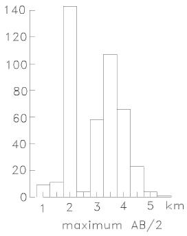
Figure 3 Histogram of the maximum half-separations between the current electrodes used in the resistivity soundings.
The transient EM soundings were acquired with the coincident-loop configuration, where a large rectangular or square loop is used as transmitter and a geometrically-coincident horizontal loop is employed as the receiver (Seismocontrol, 2005). The injected direct current (DC) in the loop is periodically interrupted in the form of a linear ramp. An induced current system, flowing in closed paths below the loop and created each time the transmitter current is interrupted, produces a secondary magnetic field. The time variation of the vertical component of this magnetic field induces a voltage in the receiving loop. As the spatial and temporal distribution of the subsurface current system depends upon the ground resistivity, the measured transient voltage gives information about the subsurface resistivity. The locus of the maximum amplitude of the induced currents diffuses downward and outward with time, thereby giving information about deeper regions as time increases (Nabighian, 1979; Hoversten and Morrison, 1982). The shape and time evolution of this induced current resembles the smoke ring of a cigarette smoker.
The area covered by the 234 TEM sounding sites is 22 km2, much smaller than the area covered by the resistivity soundings. This area is shown by an irregular blue closed box in Figure 2; for clarity, the location of the individual TEM sites has been omitted. The sites were arranged in a rectangular grid with a 300 m separation between current loops. They were acquired in 2005-2007 with a terraTEM system, employing 330 by 330 m loops. A 1 Hz repetition frequency of the bipolar current waveform was used, injecting currents of about 7.5 A. Although eight transient decays were recorded at each site, about half of them were discarded due to noisy data. Each decay curve represents the stacking of 256 individual voltage decays. Clays may produce Induced Polarization effects, usually manifested as negative voltages at late times (Smith and West, 1989). However, no evidence of this was observed in the data.
Data Modeling
The soundings were initially inverted to Occam (smooth) models and then to the traditional stratified models with a small number of layers, using in both approaches commercial software. To avoid any possible bias in the interpretation the inversions were carried out independently by three of the co-authors. A general feature of the layered models is a resistive-conductive-resistive structure under the entire study area, standing out the presence of an important conductor. An example of this general structure is shown in Figure 4, where we selected six resistivity soundings from different zones of the study area. Figure 2 shows the location of these example soundings. Each graph shows the measured apparent resistivity data with their estimated error bars, the calculated response, and the inverted model. In each sounding the observed and calculated responses are referred to the left apparent resistivity versus AB/2 electrode separation, while the right resistivity axes versus depth should be used for models. The steep decrease in the apparent resistivities responds to the presence of this unit of low resistivity. In soundings 889 and 111 the apparent resistivities display clear rises at the longest electrode separations, the inverted model then showing a deep layer of higher resistivity. In soundings 3007, 650, 601 the electrode separations were not large enough to show this climb in apparent resistivities.
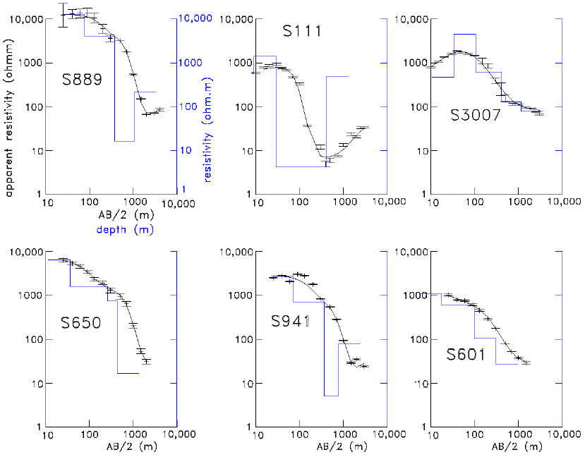
Figure 4 Selected resistivity soundings, their locations shown in Figure 2. Displayed are the observed apparent resistivities and their standard errors (symbols), the inverted layered models and their calculated responses (solid lines)
Figure 5 shows two alternative models constructed by stitching together the 1D models along profile P1; its location is described in Figure 2. Figure 5a is the section with the models initially inverted with the commercial program; Figure 5b is a reinterpretation to be described below. The layered models under each sounding site are displayed as color bars, where each color follows the scale exhibited at right. Because the resistivity values have a large range of variation, we adopted a logarithmic scale for the color compartments, with three divisions per decade. Low resistivities are denoted by hot colors (red), while cold colors (blue) are used for high resistivities. As very high resistivities have no interest in geothermal exploration, all values greater than 1,000 ohm■m are gathered into a single color compartment (dark blue). We use a vertical exaggeration of two in this section. The zero of the depth scale is at the average altitude of the profile. We also plot the position of the geothermal wells, indicating the depth interval where the geothermal reservoir is located and a simplification of the initial well temperatures estimated with the spherical-radial heat flow assumption by García Gutiérrez (2009). For reasons of clarity we do not show where the different volcanic deposits are located, however, the depth interval covered by the reservoir practically coincides with the pre-caldera volcanism lying above the basement. The locations of the TEM soundings are denoted with the letter "T".

Figure 5 Alternative resistivity sections under profile P1. a) Preliminary model, b) Reinterpreted model. The top and bottom of the conductive unit is defined by resistivities less than 100 ohm.m. Vertical exaggeration of 2x. The depth interval of the geothermal reservoir is indicated in the wells and a simplified version of the initial temperatures. The "Ts" denote the TEM soundings.
The top and bottom of the conductive unit in the sections of Figure 5 are defined by resistivity values lower than 100 ohm■m; that is, yellow, orange, and red colors. The threshold value of 100 ohm■m, although somewhat arbitrary, comes naturally from the distribution of values. In most of the soundings this conductor is directly above the reservoir, which suggests the low resistivities are due to the hydrothermal alteration clays. i.e., it is the clay cap of the conceptual model found in many geothermal systems discussed in the introduction. Mineralogical studies on drill cuttings (Prol-Ledesma, 1990; González et al., 1992; Izquierdo, 1993; Martínez and Alibert, 1994; Martínez-Serrano and Dubois, 1998) show that, indeed, at the depths of the conductive unit there are increased concentrations of montmorillonite (a subclass of smectite) and zeolites, minerals with a high CEC that produce high conductivities.
The section of Figure 5a shows several anomalous features, such as the thickening of almost 2 km of the conductor in the southwestern part of the profile and abrupt changes in the top or bottom boundaries of the conductor in the northeastern part of the model. Before attempting any interpretation of these features in terms of the structure of the geothermal system, we carried out a sensitivity analysis to estimate how well resolved are the different parameters (resistivities and layer thicknesses) of the stratified models. This approach, based on the Singular Value Decomposition (SVD) of the Jacobian matrix (Edwards et al., 1981) has been used in different geophysical studies (e.g., Verma and Sharma, 1995; Key and Lockwood, 2010; García-Fiscal and Flores, 2018) to assess which parts of the models are well constrained by the data and which are not. This approach is used only after an adequate fit between the measured and calculated responses has been reached in the inversion process. The sensitivities or Jacobians are approximated by
where
where σ is the misfit error, and
As an example of the use of this approach to our data, in Figure 6 we show it for two pairs of close-by resistivity and TEM soundings which are less than 100 m apart. Figure 6a compares the TEM sounding T24 with the resistivity sounding S954, while Figure 6b does the same for the T5 with the S3017. In the upper part the layer resistivities of the inverted models are displayed. The bars in the resistivities and depths to the layer interfaces indicate the uncertainties in these parameters. When one parameter is poorly resolved the estimated errors are extremely high. This is because the SVD technique is based on the linearization of a non-linear problem (Edwards et al., 1981). These large uncertainties are marked with an asterisk in Figure 6. The comparison between calculated and observed apparent resistivities is shown in the lower part of the figure, where symbols correspond to the measured values and their estimated standard errors displayed as error bars. The error bars in the resistivity soundings were estimated from the clutches (known as "empalmes" in Spanish), which are those apparent resistivities measured with one current electrode separation but at least two potential-electrode apertures. The errors in the TEM responses were estimated from the standard deviations of the post-stacked voltages. Notice the large uncertainties in the TEM response for late times, presumably a result of noise. From this analysis the following points can be inferred:
a)Shallow layering located at depths less than 200 m are detected and well resolved by the resistivity soundings. However, the TEM soundings distinguish only one layer in both soundings and are particularly not well resolved for the model of T5. This is an expected result because the shallow part in the transient electromagnetic soundings depends on the shortest recording time after the current shut-off (Spies, 1989), which typically was 700 microseconds. With large loops, such as those used in this study, the loop's self-inductance impedes the use of shorter times.
b) Both methods resolve fairly well the top to the conductor.
c)For the second pair of soundings (T5-S3017) the resolution of the thickness of the conductive layer is acceptable. However, for the first pair (T24-S954) the thickness and resistivity of this layer are not well resolved. This is due to an equivalence problem that affected many soundings. This problem will be discussed below.
d) The resistivity of the underlying resistive unit sometimes is well resolved by the VES; however, the TEM soundings do not resolve this parameter.

Figure 6 Comparison of inverted models and parameter resolution between a pair of close-by transient electromagnetic (TEM) and resistivity soundings. a) Soundings T24 and S954, b) soundings T5 and S3017. Large uncertainties (low resolution) are indicated with an asterisk. The measured apparent resistivities and standard errors as a function of electrode aperture or time are displayed in the lower part, together with the calculated response from the inverted model.
This equivalence problem is illustrated with sounding S109 in Figure 7 where four possible models are displayed. These models have the same conductance (the ratio of thickness over resistivity) in the low-resistivity layer but the individual resistivity and thickness are different. The apparent resistivity responses from the four models are shown in the right panel, the differences between them are so small that they cannot be differentiated. According to Orellana (1972), the equivalence in the conductance of a layer occurs with thin and low-resistivity layers, particularly, when the layer transverse resistance (the product of thickness by resistivity) is much less than the cumulative transverse resistance of all the overlying layers. For this model, the cumulative resistance is more than 35 times greater than the resistance of the conductive layer. Then, the practical consequence of this equivalence problem is that there are many pairs of thickness and resistivity of this layer that fulfill the data; it is a non-uniqueness problem, common to several geophysical methods.
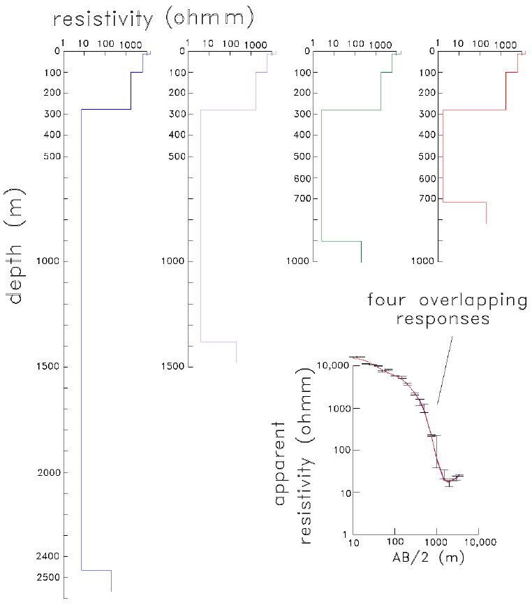
Figure 7 Equivalence problem in the resistivity sounding S109. Four models with the same conductance of the fourth layer produce practically the same apparent resistivity responses. The field data are also shown.
Information external to the geophysical method has to be used to solve the equivalence problem. Over the reservoir, the well temperatures and their associated hydrothermal alteration were employed to constrain the base of the conductive zone. As mentioned above, the conductive clay-cap is produced by the presence of smectite and illite, hydrothermal minerals occurring at temperatures between 70° and 200°C. Then, in Figure 5b the bottom of the conductive zone was set at the depth corresponding to the vicinity of 180°C, where these two argillic minerals show a gradual content decrease. For soundings not located over the reservoir, we constrained the models to have a smooth lateral variation in the top and bottom of the conductive unit, done by trial and error in a site-by-site basis. This reinterpretation process for the resistivity soundings was carried out in about 45% of the soundings with an in-house non-linear inversion program based on the algorithm proposed by Jupp and Vozoff (1975) which considers the standard deviation of the data, something that the commercial program ignores. It is important to emphasize that the two models of Figure 5 reproduce the observed data equally well, such that both of them are valid. However, we prefer the second model (Figure 5b) because it is constrained by a priori information. In the first model (Figure 5a) anomalous features in the model could have been given geothermal significance when the equivalence problem in fact produces them.
The same two constraints mentioned above were applied to the four profiles of Figures 8 and 9. Profiles P2, P3, and P5 have a NW-SE azimuth, P4 is SW-NE; their locations are indicated in Figure 2. Profile P5 is the only one not passing over the production zone. From these models (Figures 5b, 8, and 9) we can infer the following general features:
a) The top of the clay cap tends to be shallower over the reservoir;
b) The resistivity of the clay cap tends to be lower over the reservoir;
c) The clay cap not only occurs over the geothermal reservoir (as in Figure 1) but is present under the whole area of study.
d) Not all measurements sensed the top of the deep resistive unit; soundings with half-separations of 2 km or less, such as soundings 601 and 650 of Figure 3, could not detect the resistive layer underlying the clay cap.
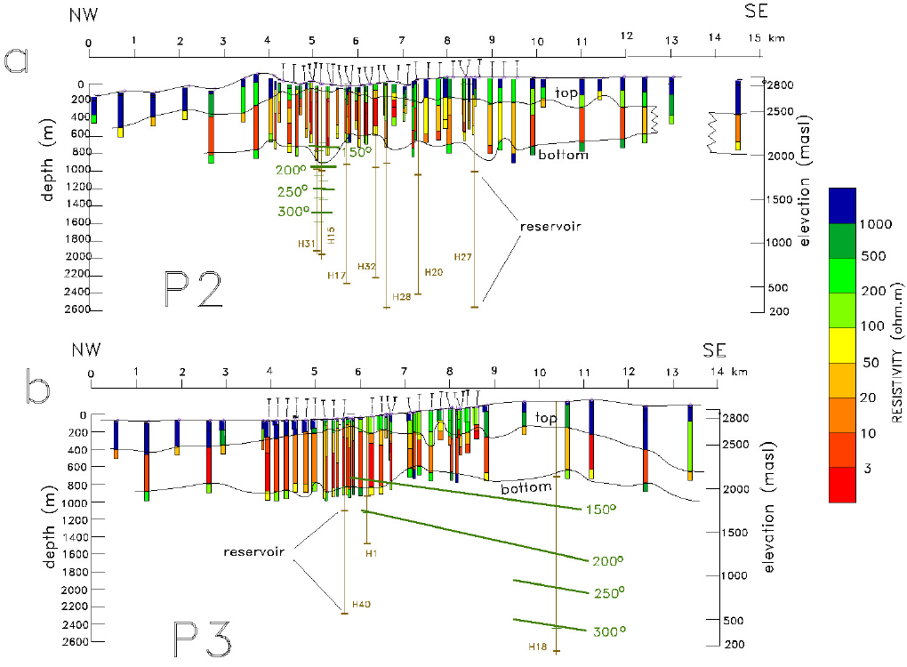
Figure 8 Reinterpreted models constructed for the NW-SE profiles P2 and P3. Profile locations are shown in Figure 2. The top and bottom of the conductive unit is defined by resistivities less than 100 ohm.m. Vertical exaggeration of 2x. The geothermal reservoir is indicated in the wells and a simplified version of the initial temperatures. The "Ts" denote the TEM soundings

Figure 9 Reinterpreted models constructed for profiles P4 (SW-NE) and P5 (NW-SE). Profile locations are shown in Figure 2. The top and bottom of the conductive unit is defined by resistivities less than 100 ohm.m. Vertical exaggeration of 2x. The geothermal reservoir is indicated in the wells and a simplified version of the initial temperatures. The "Ts" denote the TEM soundings.
Map Distribution O Model Parameters
We now turn to analyze the horizontal distribution of the resistive-conductive-resistive structure. Here we will focus on the results from the resistivity soundings because of its greater areal coverage. It is worth mentioning that the parameters are quite irregular, however, global trends can be drawn. The shallow resistive unit is made by up to five layers, but two and three layers contribute 87% of all the models. The average thickness of this unit is 240 m. To obtain an equivalent resistivity

Figure 10 Equivalent resistivity of the shallow resistive unit. Red zones enclose values less than 1,000 Om. The main faults are also depicted.
Another interesting feature is that there is no evidence of a continuous low-resistivity zone within this resistive unit that could be associated with an aquifer, as is usually the case in a sedimentary basin. This is supported by eight exploration wells reported by Cedillo (1999) (maximum depths from 210 to 360 m), four of them located inside the Los Humeros Caldera and four outside. Only in five of them a phreatic level was detected but at significantly different depths. This suggests they are associated with local aquifers because the regional piezometric surface could not be defined. This indicates that secondary permeability is the controlling factor in the resistive unit.
In the profiles above we noticed that the depth to the top of the conductive unit apparently is shallower where the reservoir is located. Figure 11 shows the spatial behavior of this unit displayed by the depth contours of 200 and 400 m below the surface. Depths shallower than 200 m occur mainly over the production zone. The other zone with shallow depths is located in the southwestern corner of the study area. If a direct relationship exists between a shallow clay cap and the presence of a geo-thermal reservoir, it would be worth to further explore this southern zone. An alternative explanation for this zone is that an old thermal episode produced the hydrothermal clay alteration but now the temperatures are not sufficiently high for the existence of a geothermal reservoir. The mean resistivity of the conductive unit is 8.7 +/- 6.8 ohm■m.

Figure 11 Depths to the top of the conductive unit. Red areas: depths less than 200 m; green areas: depths between 400 and 200 m. The locations of e main faults are also shown.
Figure 12 shows the conductance of this conductive unit where values greater than 100 Siemens are enclosed by the red contour and are mainly concentrated above the reservoir. It is worth noting the high lateral variability of this parameter, which could be explained by the formation in vertical fractures and faults of the alteration clays.
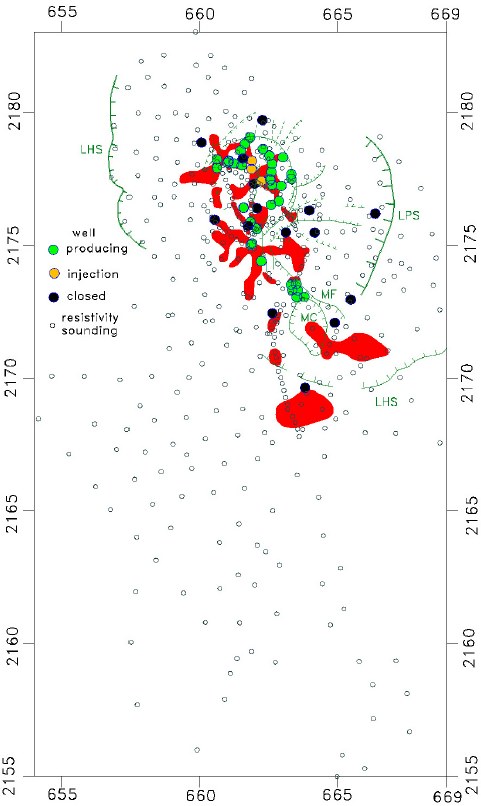
Figure 12 Conductances of the conductive unit higher than 100 Siemens are displayed in red. The locations of the main faults are also shown.
One last subsurface parameter we analyze is the resistivity of the layer below the clay cap, that is, the deep resistive unit. Many soundings either could not detect this unit or they did not have enough points in the ascending apparent resistivity data to adequately resolve this resistivity. In these cases, the maximum electrode separations of the Schlumberger soundings were not large enough to reach greater depths of investigation. Examples of these responses are soundings 650, 941, and 601, shown in Figure 4. However, 26 soundings rendered models with a deep resistivity reasonably well resolved, such as that of sounding 111 (Figure 4). In this group, the average depth to the top of this deep resistive unit is 600 m. By employing a perturbation analysis on several of these models we estimate this unit extends to depths of the order of 2 km. For this analysis we assumed the presence of an additional test layer with a starting depth to its top of 5 km and resistivity two times or half the value of the deep resistive unit. We then decreased in steps the depth of this test layer, calculating the apparent resistivity response in each step. When the depth was about 2 km the apparent resistivities of the largest electrode separations started to fall beyond the error bars of the measured response, suggesting this as the maximum depth of investigation of these soundings.
The deep resistivities and corresponding uncertainties of the 26 models are displayed in Figure 13. They are sorted into two groups: on the left side of this figure are 16 soundings falling in the drilled area, on the right side are 10 soundings located more than 2 km away from any nearby well. Additionally, the first 11 values of the left group (soundings 88 to 3082) correspond to those located less than 500 m from a producing well, the remaining five soundings do not have a close producing well. The logarithmic means of the three resistivity groups (109, 141, and 150 ohm■m) and the corresponding uncertainties (defined by +/- one standard deviation) are indicated in this figure with the horizontal lines. Because the uncertainties overlap, statistically the average resistivities of the three groups are indistinguishable from each other. The average value of the 16 soundings within the drilled area is 118 ohm■m.

Discussion
The resistivity structures inferred from neighboring VES and TEM soundings are similar but rarely are the same. Several factors may explain these differences, among them is the different attitudes the electric currents have in the subsurface; while in the TEM method the induced currents tend to be horizontal, in the DC galvanic technique the injected currents have both horizontal and vertical components. They also have different depths of investigation. For example, in shallow depths the VES can distinguish vertical resistivity changes in the first few meters, while the shallowest interface the TEM soundings can detect is of the order of 200 m (Spies, 1989). Furthermore, the lateral dimensions of the subsurface volume that contributes to a given surface voltage measurement are different; in the TEM soundings the maximum lateral dimensions are of the order of several hundred meters, while in the VES soundings, depending on the maximum AB/2 electrode separation, they can reach several kilometers. Therefore, the TEM soundings are expected to have a better lateral resolution.
The resistivity and TEM data could, at least in theory, be inverted to a 3D model. However, this is a difficult task for the large size of the matrices involved in the inversion. For example, assuming the use of a finite differences inversion approach, would require defining grid nodes at each of the current and potential electrodes, which would require at least 22,000 nodes to model all the VES data; the size of the resulting matrices would be hard to handle. Furthermore, the coordinates of the center of each sounding are known, but not the required x,y position of the electrodes.
The recharge zone, where meteoric water percolates and feeds the deep hydrothermal fluids, is an important component of any conceptual model of a geothermal field. There are two trends on where the recharge zone is located. Cedillo Rodríguez (1999) suggests a local recharge zone situated within the Los Humeros caldera, where the various mapped faults work as the downward conduits of rainwater. Other studies (Yáñez, 1980; Pinti et al., 2017; Les Landes et al., 2020; Lelli et al., 2021) support a regional recharge from the nearby outcropping Mesozoic limestones of the Sierra Madre Oriental. Figure 10 outlines the areas where the shallow resistive unit has equivalent resistivities less than 1000 ohm m. They occur mainly over the geothermal field and a large zone in the southern edge of the study area; their decreased resistivities could be produced by the presence of water in enhanced permeability zones, which could represent recharge zones. The low resistivity zone in the vicinity of the reservoir would favor the proposal of Cedillo Rodríguez (1999) of a local recharge zone, while the region in the southern limit of the study area would suggest a regional recharge zone. As we do not have any sounding over the Mesozoic calcareous rocks, we cannot estimate the possible contribution to the recharge from this type of outcrops.
The results displayed in Figure 13 are important for the search of a link between the deep resistivity and the presence of the geothermal reservoir. In this figure we sorted the deep resistivities according to the distance to a drilled well. In the first group are those soundings located less than 500 m from a productive well, in the second, those positioned within the drilled area but more than 500 m from any productive well, and in the third those situated outside the drilled area and more than 2 km from any nearby well. The lower average value of the first group (109 ohm■m) with respect to those of the second (141 ohm■m) and third (150 ohm■m) groups could be interpreted as the effect of hot and saline fluids residing in the near-vertical fractured rocks of the geothermal reservoir, decreasing the rock resistivity. Unfortunately, the uncertainties of the inverted resistivities and the overlapping of the standard deviations of the average values (Figure 13) preclude confirming such correlation. The higher mean value of the third group (150 ohm■m) with respect to those of the first and second groups could be due to an absence of hot geothermal fluids. But again, these resistivities are not statistically different, such that this claim cannot be assured.
Assuming that 8 km south of the drilled area (where sounding 657 is located) there is no geothermal reservoir, the deep resistivity value of 303 ohm'm obtained for this sounding (Figure 13) could be produced by the presence of chlorite, a hydrothermal alteration mineral that decreases the resistivity, but not to the extent as lower temperature minerals such as smectite does. The presence of this intermediate resistivity, together with the generalized occurrence of the conductive unit suggests the existence of one or several thermal events that produced this regional presence of alteration minerals.
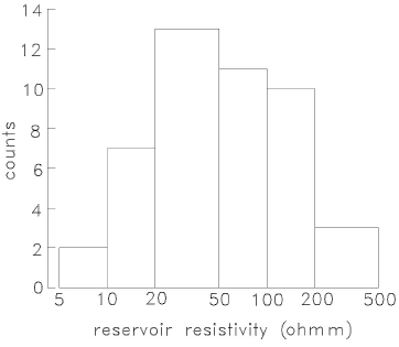
The average value of 109 ohm■m of the resistive unit representing the reservoir is higher than the upper limit of 60 ohm■m proposed by Pellerin et al. (1996) in their conceptual model depicted in Figure 1. To test how common is this 10 to 60 ohm■m interval for the so-called resistive core, we carried out a survey of published literature in geothermal fields around the world that report wells with temperatures of at least 200 °C and estimated resistivities at these depths, the result of inversion of geophysical data (usually with the magnetotelluric method). We found published papers on 28 geothermal fields that fulfilled these two requirements. The results are shown in Table 1 and displayed in Figure 14 as a histogram with three resistivity divisions per decade. Although the most common occurrence is from 20 to 50 ohm■m, geothermal fields with reservoir resistivities from 100 to 200 ohm■m are not uncommon. Then, the mean value of 109 ohm■m for the Los Humeros reservoir resistivity cannot be considered anomalous.
Table 1 Estimated reservoir resistivities in geothermal fields around the world.
| Geothermal field | resistivity (Ωm) | Source |
|---|---|---|
| Hengill, Iceland | ~ 150 | Arnasson et al., 2010 |
| Ohaaki, New Zealand | 50 to 100 | Bertrand et al., 2012 |
| Aluto-Langano, Ethiopia | 20 to 50 | Cherkose & Mizunaga, 2018 |
| Glass Mountain, USA | 100 to 150 | Cumming and Mackie, 2010 |
| Krafla, Iceland | 30 to 80 | Gasperikova et al., 2011 |
| Namora, Indonesia | 8 to 25 | Gunderson et al., 2000 |
| Awibengkok, Indonesia | 15 to 30 | Gunderson et al., 2000 |
| Rotokawa, New Zealand | ~ 100 | Heise et al., 2008 |
| Krýsuvík, Iceland | 3 to 200 | Hersir et al., 2020 |
| Northern Negros, Philippines | 20 to 60 | Layugan et al., 2005 |
| Southern Leyte, Philippines | 40 to 100 | Layugan et al., 2005 |
| Mahagnao, Philippines | 30 to 60 | Layugan et al., 2005 |
| Coso, USA | 40 to 200 | Lindsey et al., 2017 |
| Mahanagdong, Philippines | 20 to 50 | Los Baños & Maneja, 2005 |
| Travale, Italy | 200 to 500, 250 & 60 to 90 | Manzella et al., 2010 |
| Tolhauaca, Chile | 30 to 60 | Melosh et al., 2010 |
| Mutnov, Russia | 60 to 100 | Nurmukhamedov et al., 2010 |
| Lahendong, Indonesia | 15 to 40 | Raharjo et al., 2010 |
| Kamojang, Indonesia | 50 to 150 | Raharjo et al., 2010 |
| Irruputuncu, Chile | ~ 20 | Reyes et al., 2011 |
| Asal, Djibouti | 26 | Sakindi, 2015 |
| Aluto-Langano, Ethiopia | 10 | Samrock et al., 2015 |
| Sumikawa, Japan | 100 to 200 & 300 | Uchida, 1995 |
| Mataloko, Indonesia | 100 to 200 & 300 | Uchida et al., 2002 & Uchida,2005 |
| Ogiri, Japan | 200 | Uchida, 2010 |
| Yanaizu-Nishiyama, Japan | 10 to 30 | Uchida et al., 2011 |
| Takigami, Japan | 100 to 200 | Ushijima et al., 2005 |
| Sabalan, Iran | 20 to 30 | Talebi et al., 2005 |
| Dixie Valley, USA | 70 to 200 & ~ 100 | Wannamaker et al., 2007 |
It is interesting to compare the deep resistivities at reservoir depths estimated with the VES soundings with those obtained with the Magnetotelluric (MT) method. There are two MT field data, those acquired in the CeMie-GEO project (Arzate et al., 2018), and those measured in the GEMex project (Benediktsdóttir et al., 2020). They have been interpreted using 1D (Romo-Jones et al., 2020), 2D (Arzate et al., 2018), and 3D inversion approaches (Corbo-Camargo et al., 2020; Benediktsdóttir et al., 2020; Romo-Jones et al., 2021). Focusing in the 3D results, it is not easy to carry out comparisons between the modeled resistivities because the analyzed profiles in these works are different. However, the models close to producing wells can be compared. In the vicinity of productive wells H-7 and H-8 the resistivities in the depth range of the reservoir are: 50 to 200, 15 to 170, and 15 to 120 ohm'm given, respectively, by Corbo-Camargo et al., 2020, Benediktsdóttir et al., 2020, and Romo-Jones et al., 2021. Close to another productive well H-19, the resistivities are about 200, 15 to 50, and 5 to 200 ohm■m, respectively, from the same articles in the same order. Although there are obvious differences between the MT results and also with our results (50 to 220 ohm■m, Figure 13), the ranges of variation overlap in several cases.
Conclusions
With the interpretation of DC resistivity and transient electromagnetic soundings we found a global resistive-conductive-resistive vertical sequence. The shallow resistive unit has an average thickness and resistivity of 240 m and 1600 ohm■m, respectively. There are two low-resistivity zones within this unit, over the reservoir and in the southern region; these might be recharge zones where the downward circulation of meteoric water feeds the reservoir.
The resistivity and thickness of the conductive unit, interpreted as the clay cap, cannot be estimated separately due to an equivalence problem. This was circumvented by using the well temperatures and their association with the argillic hydrothermal alteration. The average thickness and resistivity of this unit are 440 m and 7.4 ohm■m, respectively. The depth to the top tends to be shallower and their resistivities have lower values over the reservoir. We propose that these features could be used as proxy indicators of a geothermal reservoir in other prospective areas. The conductive unit appears under the whole studied area, indicating a regional hydrothermal alteration, possibly resulting from several thermal events.
In 26 VES models the resistivities of the third unit were well resolved with reasonable small uncertainties; these depths correspond to where the geothermal reservoir lies, with average values from 100 to 150 ohm■m. The resistivities close to productive wells have average values slightly lower than those far from the wells, unfortunately their uncertainties overlap, such that they are not statistically different from each other. There are partial agreements between our resistivities and those estimated from previous magnetotelluric inversions. To examine how common is our estimated range of resistivities compared with other geothermal fields in the world, we searched for published studies with wells with temperatures over 200 °C and estimated reservoir resistivities with geophysics, finding 28 of them. Our range of 100 to 150 ohm■m is not the most frequent, but represents a significant 36% of all the cases.

