


 nueva página del texto (beta)
 Inglés (pdf)
 Artículo en XML
 Referencias del artículo
 Enviar artículo por email
 Citado por SciELO
  Similares en
SciELO
Similares en
SciELO 
 Permalink
Introduction
Gravity investigation plays an important role in geological studies and has been used widely over the years for modeling buried geological structures and deposit, especially in mineral reconnaissance projects. The non-uniqueness in the linear inverse problem of gravity, i.e., the existence of a large variety of distribution of subsurface density distribution models that generate a similar gravity effect on measurement plane, makes one to hesitate on the reliability of solution (Skeels, 1947; Parker, 1972). In order to obtain a correct unique solution and to decrease the ambiguities, various researchers have been proposed different algorithms to increase the amount of extracted information from inversion for simulating the geometry of a density distribution related to a known gravity anomaly, such that the proposed model be geologically realistic.
Tsuboi (1983) introduced a simple but effective approach based on the equivalent stratum technique to estimate 3D topography of a density interface. Oldenburg (1974) proved that the Parker's expression could be applied in order to specify the geometry of the density interface from its gravity anomaly. The geological maps and petrophysical data from rock samples were used to constraint the model parameters to realistic values (Farquharson et al., 2008; Williams, 2008; Heincke et al., 2010; Lelièvre et al., 2012; Tschirhart et al., 2013, 2017). Kamm et al. (2015) used the petrophysical information conduct a joint inversion of gravity and magnetic data. Ialongo et al. (2014) show that there are invariant models in the inversion of gravity and magnetic fields and their derivatives.
Using a joint inversion of multiple data sets can also diminish the nonuniqueness of the inverse problem. examples of joint inversion of gravity and magnetic data are given by, e.g., Zeyen and Pous (1993), Gallardo and Meju (2003), and Pilkington (2006) using deterministic inversion techniques and by Bosch and McGaughey (2001), Bosch et al. (2006) and Shamsipour et al. (2012) using stochastic methods. Shamsipour et al. (2010, 2011, 2012) proposed geostatistical techniques of cokriging and conditional simulation for the separate three-dimensional inversion of gravity and magnetic data respectively, including geological constraints.
One way to eliminate the inherent ambiguity is to propose a geologically sound geometry as the source of the anomalous body with a known density as the start point of the inversion of gravity anomalies (Chakravarthi and Sundararajan, 2004). Although simple models may not be geologically realistic, they usually are sufficient to analyze sources of many isolated anomalies (Abdelrahman and El-Araby, 1993). The interpretation of a given anomaly aims essentially to estimate the parameters such as shape, depth, radius, thickness and so on. Thus, in this case it is dealed with nonlinear inverse modeling. The many of the proposed nonlinear techniques are based on an initial guess of the geological structure parameters, 1) in the case of least-squares minimization approaches (Gupta, 1983; Lines and Treitel, 1984; Abdelrahman, 1990; Abdelrahman et al., 1991; Asfahani and Tlas, 2007, 2008) 2) different neural networks (Eslam et al., 2001; Osman et al., 2006 and 2007; Al-garni et al. , 2013; Eshaghzadeh and Kalantari, 2015; Eshaghzadeh and Hajian, 2018); 3) Continual least squares methods (Abdelrahman and Sharafeldin 1996; Abdelrahman et al. 2001, 2001a, 2001b; Essa 2012, 2013); 4) effective quantitative interpretations using the least-squares method based on the analytical expression of simple moving average residual gravity anomalies (Gupta, 1983; Abdelrahman et al. 2003, 2007, 2015). Appraisal of the depth and shape of a buried structure from the observed gravity and gravity data is widely used in exploration operations, in methods based on the Fourier transform (Odegard and Berg, 1965; Sharma and Geldart,1968); Mellin transform (Mohan et al. 1986); Walsh transforms techniques (Shaw and Agarwal, 1990); ratio techniques (Hammer, 1977; Abdelrahman et al. ,1989; Cooper, 2012; Eshaghzadeh, 2017).
Dyke is a sheet-like geological structure generated from intrusive igneous rock while cut through the strata. Dyke structure has different slopes, thicknesses and lateral dimension extent. Structures that have a higher density contrast than that of thier encasing formation as are easily detectable in the residual gravity field maps. Because of existence the important minerals in the igneous rock, such as chromite, magnetite and so on, these tabular structures are among the very considerable exploratory targets in geophysical investigations, especially when based on potential fields methods.
By searching many papers related to our subject it can be found that their focus is on determining the parameters of dyke-like gravity sources (Bastani and Pedersen 2001; Abdelrahman and Essa 2007; Abdelrahman et al. 2003, Asfahani and Tlas 2007; Tlas and Asfahani 2011a, b; Cooper 2012, 2014, 2015; Abdelrahman et al. 2015) while it can be stated that dyke non-linear inverse modeling from gravity data less has been investigated. Ateya and Takemoto (2002) proposed a gravity inversion modeling across a 2-D dike-like structure. A fast simulated annealing global optimization technique has been proposed by Biswas (2016) to the interpretation of gravity and gravity anomaly over thin sheet-type structure. Biswas et al. (2017) also applied a nonlinear optimization method for the determination of dyke-type source parameters based on the calculation of first order horizontal and vertical derivatives of the gravity and gravity anomalies. Peace et al. (2018) employed the full tensor graviometry (FTG) data for 3-D subsurface models of the Budgell Harbour Stock and associated dykes, Newfoundland, Canada. Abdelfattah et al. (2021) performed an integrated analysis based on gravity and seismological data with focusing on the HL seismogenic and volcanic zone in the western shield of Saudi Arabia, which has a complex structure comprises dykes, recent volcanic eruptions, and fault segments of various orientations.
For first one, in this study, we employ the linear inverse modeling technique based on the damped singular value decomposition (DSVD) and using a depth weighting parameter as resolution enhancer and a two-norm (also known as the L2 norm or least squares) as stopping criteria in inversion algorithms. SVD constitutes a famous and numerically stable method for analyzing the underdeter-mined problems, i.e. ill-condition matrices, and is a standard technique for small inverse problems.
We also develop the Marquardt's algorithm (1963) for inverting the 2-D observed gravity anomaly due to finite dyke-shape model in order to evaluate the depth to top, height (the depth to bottom is estimated), width and slope of buried structure. We exemplify the capability of the both methods by a theoretical model with and without a random noise. Finally, these inversion techniques are employed for the interpretation of the real gravity data from Iran.
Computing the kernel matrix
For inverting the gravity data for calculating a 2D density distribution, it is necessary that the subsurface be divided in order to calculate the gravity effect of the obtained density distribution at the surface. For a 2D model, as shown in Figure 1, the gravity effect of all the rectangular blocks at the observation point i, is given by:
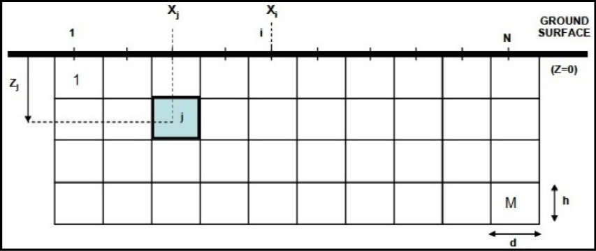
Figure 1 A 2-D schematic view of the inversion domain divided into several blocks as the gravity stations are located at the center of the blocks at the ground surface.
where M and N denote the number of blocks and the number of observations, respectively,
Where
And
Here G is the gravitational constant, d and h are the width and height of each block.
Linear inversion methodology
In most of the inverse modeling cases, we deal with the underdetermined problems, i.e. the number of unknowns is much greater than the number of observed data. For a general underdetermined system of linear equations, i.e. d=Pf where d is the column vector of the observed gravity field data, f is the column vector of the unknown, i.e. density, and P is the kernel rectangular matrix, the minimum norm solution is defined as the model that fits the data exactly which is given by (Menke, 1984):
we can solve the inversion problem using the standard damped least-squares method, as:
where γ is the damping parameter or regularization parameter, I is an identity matrix and the superscript T denotes the matrix transposition. The solution of equation (4) can be estimated by minimizing the following Tikhonov cost function:
Analyzing this expression can be realized that the duty of the damping is minimizing the first term of equation (5) values to finding the model that gives the best fit to the data to Minimize the last term values to obtain the model with the smallest norm. The choice of γ is usually determined by trial-and-error.
In order to stabilize the inversion, the singular value decomposition (SVD) technique is usually employed. The equation for singular value decomposition of matrix
where S is an n × m left eigenvector matrix, U is an n × n diagonal matrix. The elements of
Therefore, we can rewrite the equation 3 as:
The singular value decomposition of matrix
where r is the rank of matrix
On the basis of equation (10), the damped least-squares solution (equation 4) can be rewritten as the damped SVD, we will have:
Here
Usually, in the first iteration, the regularization parameter is considerated to be a large positive value as at each iteration the damping factor is multiplied by a factor less than unity so that the least-squares method reaches near a solution (Meju, 1994). According to Arnason and Hersir (1988) the damping factor is determined as follows:
Where R is the iteration number for the damping factor at any iteration, s is the eigenvalue parameter and the term Δd is given by
Where,
In inverting gravity data due to a causative mass, the evaluated density distribution related to a buried structure tend to concentrate near the surface. For nullifying the natural decay of the kernels and maximizing the depth resolution, a depth weighting function is included in the problem. Li and Oldenburg (1998) suggested to employ a depth weighting function such as:
where z is the depth of the layers and
In this paper, we employ the two-norm (L2 norm) as a criterion for stopping the iteration process in the inversion algorithms. The L2 norm has the form:
Where the e is the difference between the observed gravity data and inverted gravity data due to the evaluated model from the density distribution at each iteration. The best form of the under surface density distribution is obtained when the L2 norm in an iteration achieve the value less than the predefined value which in this case the iteration is terminated. Otherwise, the lowest amount estimated by the L2 norm during inversion process is considered as the best inverted under surface density distribution.
Synthetic model analysis with damped SVD
Figure 2(a) shows the gravity response due to the assumed model shown in Figure 2(b) where the subsurface ground has been partitioned into 15 × 10 prisms with the respective dimensions of 10 m × 5 m. As is shown in Figure 2(b), the 2D model include 6 prisms whose density contrast is 1000 kg/m3. The gravity effect corresponding to the resulting inverted causative body (Figure 2c), is displayed in Figure 2(a). This inverted model that is exactly similar to the original causative body, was obtained at 5th iteration, where the L2 norm as the stopping criterion attain the smallest amount.
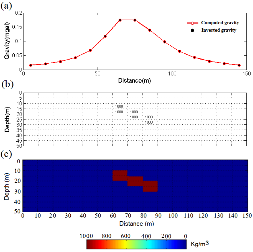
Figure 2 a) Computed and inverted gravity due to b) first assumed synthetic model and c) inverted model, respectively.
For testing the stability and sensitivity of the inversion method, we divided the subsurface inversion domain, Figure 2(b) into 75 × 25 blocks of dimension 2 m × 2 m (Figure 3). Therefore, the whole domain is 150 m × 50 m and the total number of blocks is M=1875.
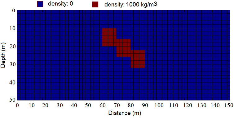
Figure 3 Second assumed density model in the inversion domain, which is constituted by 75 × 25 blocks with dimension 2 m × 2 m.
Figure 4 shows the inferred density distribution from inverse modeling. The effect of error has been studied by adding 5% of random noise to the gravity response of the model shown in Figure 3. The inversion result is presented in Figure 5. These inverted models, i.e. figures 4 and 5, accrue at 7th and 10th iterations, respectively. Since, the inverted structures in both cases, with and without noise, are close to that of the assumed model, it can be concluded that the damped SVD inversion provides satisfactory results.
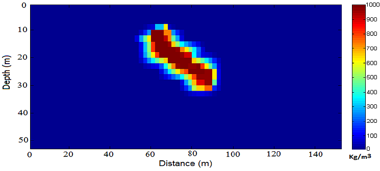
Figure 4 The obtained density distribution from inverting the gravity response of the second assumed model.
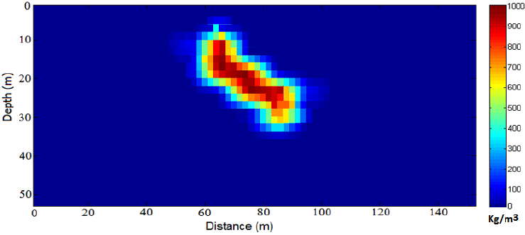
Gravity of dyke model
The gravity effects g(i) of a finite dyke-like structure at a point x(i) along a profile perpendicular to its strike direction which runs across the center of the target (Figure 6), is given in Telford and Geldart (1976) as
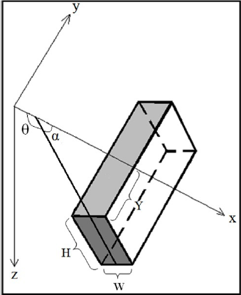
Where the G is the gravitational constant, ρ is the density contrast, w is the thickness, θ is the dip angle of the dyke considered anticlockwise from horizontal, z is the depth to the top, 2Y is the strike length of the dyke and H is the dipping extent of the buried dyke.
Nonlinear inversion methodology
The inversion of gravity anomalies is implicitly a mathematical process, aimed at fitting the computed gravity anomalies to the observed ones in the least-squares approach and then estimating the four parameters namely the depth to top (z), width (thickness) (w), dip (slope) θ and dipping extent (height) (H). The process of the inversion begins by computing the theoretical gravity anomaly of the assumed simple geometry using equation (17). The difference between the observed gravity
N is the number of observed gravity data. We have employed the Marquardt's algorithm (1963) given by Chakravarthi and Sundararajan (2006a) for minimizing the misfit function until the normal equations can be solved for overall modifications of the four unknown structural parameters, as
where
and λ is the damping factor. The advancements, dak, k=1, 2, 3 and 4 evaluated from equation (19) are then added to or subtracted from the available parameters estimated from last iteration and the process repeats until the misfit, J, in equation (18) descends below a predetermined allowable error or the damping factor obtains a large value which is greater than predefined amount or the repetition continues until the end of the considered number for iterations (Chakravarthi and Sundararajan, 2008).
Synthetic model analysis with Marquardt inversion
Figure 7(a) show the observed and calculated gravity anomalies due to the initial and assumed models which are shown in figure 7(b). The considered values for the density contrast is ρ = 1000 kg/m3 and semi-length of the dyke strike is Y=50 m, values that during inversion remain constant. The selected values for the parameters which improve during inversion, i.e. depth to top, width, dip and height for the initial model are 20 m, 15 m, 60° clockwise from the horizontal toward the right (i.e. α in Figure 1 or 120° anticlockwise from the horizontal (θ)) and 60 m, respectively and for the assumed model are 15 m, 12 m, 54° clockwise from the horizontal (i.e. α in Figure 6 or 36° from the vertical to the right) and 51 m, respectively.
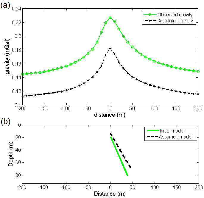
Figure 7 a) The observed and calculated gravity anomalies along a profile due to b) the initial (z=20 m, w=15 m, α=60 degree and H= 60 m) and assumed (z=15 m, w=12 m, α=54 degree and H= 51 m) models with a density contrast of 1000 kg/m3
The predefined values for misfit function, J, iteration number and maximum damping factor (λ) are 10-4 mGal, 100 and 14, respectively. The initial damping factor is given as 0.5.
The misfit, J, reduces intensely from its initial value of 0.214 mGal at the first iteration to 0.000073 mGal at the end of the 6th iteration and then incrementally reaches 45 × 10-7 mGal at the 10th iteration (Figure 8e). Because the misfit, J, obtained at the 10th iteration was smaller than the allowable error value, the iteration process is ceases and therefore the optimum estimates for the depth, width, dip and height (dipping extend) are corresponding to the evaluated quantity at 9th iteration of the inverse modeling.
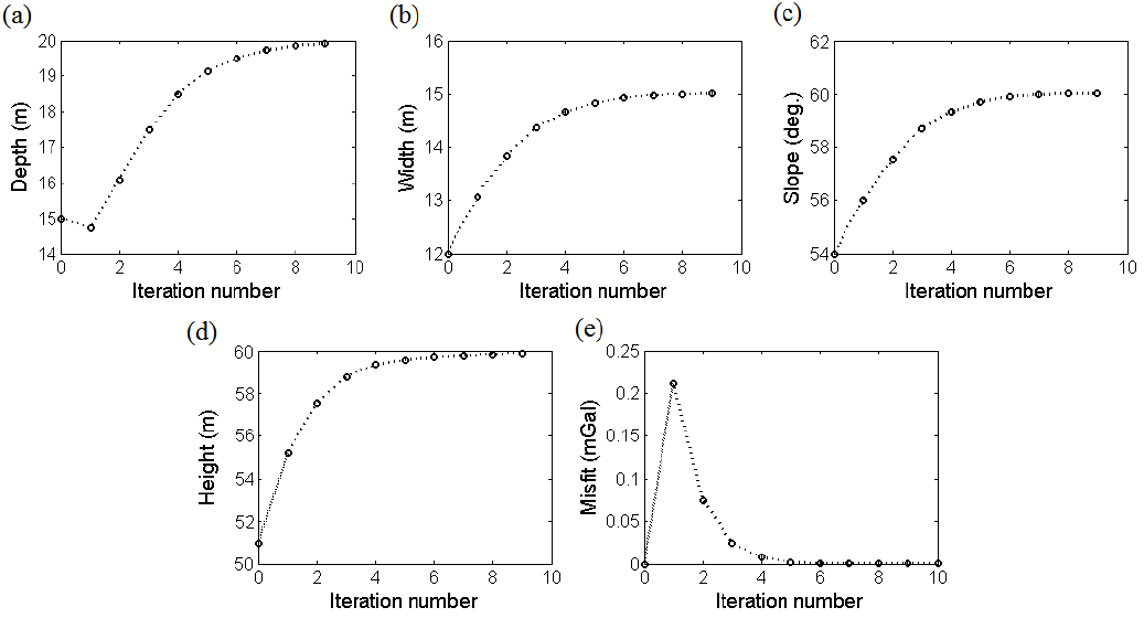
Figure 8 The variations of a) depth b) width c) dip d) height and e) misfit function versus iteration number for synthetic gravity data in figure 2.
Figures 8(a), 8(b), 8(c) and 8(d) shows the variations of the model parameters, i.e. z, w, α and H versus the iteration number. The conclusive obtained parameters values are z=19.98 m, w=15 m, α=60.01 degree and H=59.97 m.
Figure 9(a) exhibits the inverted gravity anomaly from the resulted model parameters which is shown in Figure 9(b). The percentage of error in the determination of the depth, width, dip and height parameters are 0.1, zero, about 0.017 m and 0.05, respectively. The considered parameters values and numerical results for the synthetic gravity data are tabulated in Tables 1.
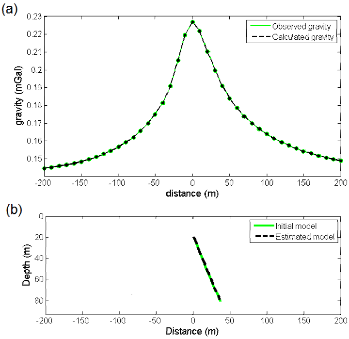
Figure 9 a) The observed and calculated gravity anomalies along a profile due to b) the initial (z=20 m, w=15 m, α=60 degree and H=60 m) and estimated (z=19.98 m, w=12 m, α=60.01 degree and H= 59.97 m) models with a density contrast of 1000 kg/m3
Table 1 Numerical results obtained from the Marquardt inversion of the synthetic gravity data
| Parameter | Depth (m) | Width (m) | Dip α (degree) | Height (m) |
|---|---|---|---|---|
| Initial | 20 | 15 | 60 | 60 |
| Assumed | 15 | 12 | 54 | 51 |
| Estimated | 19.98 | 15 | 60.01 | 59.97 |
| Error % | 0.1 | 0 | 0.017 | 0.05 |
| Iteration | 9 | |||
| Misfit (mGal) | 62 × 10-7 | |||
The effect of error has been evaluated by adding 10% random noise to the gravity response of the initial dyke model (Figure 7a) using the following expression:
where
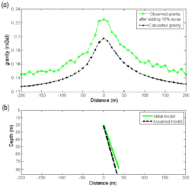
Figure 10 a) The observed gravity anomaly with a added random noise of 10% and calculated gravity anomaly along a profile due to b) the initial (z=20 m, w=15 m, α=60 degree and H= 60 m) and assumed (z=22 m, w=13 m, α =63 degree and H= 63 m) models with a density contrast of 1000 kg/m3
In noisy data case, the assigned values for misfit function, J, iteration and maximum damping factor (λ) are set as in the free-noise data case. The initial damping factor also is determined as 0.2.
The misfit, J, reduces quickly from its initial value of 0.0493 mGal at the first iteration to 0.0024 mGal at the end of the 5th iteration and then incrementally attains 0.0057 mGal after the 16th iteration (Figure 11e). The iteration finished at the 16th iteration where the damping factor value exceeded from the predefined value and reached a value of 24.62. The final values of the evaluated depth to top, width, dip and height at the 15th iteration are z=19.9 m, w=14.7 m, α=62.08 degree and H=61.5 m, respectively (Figures 11a to 11d). The percentage of error in the estimation of the depth to top, width, dip and height are 0.1, 2, about 3.67 and 2.5, respectively.
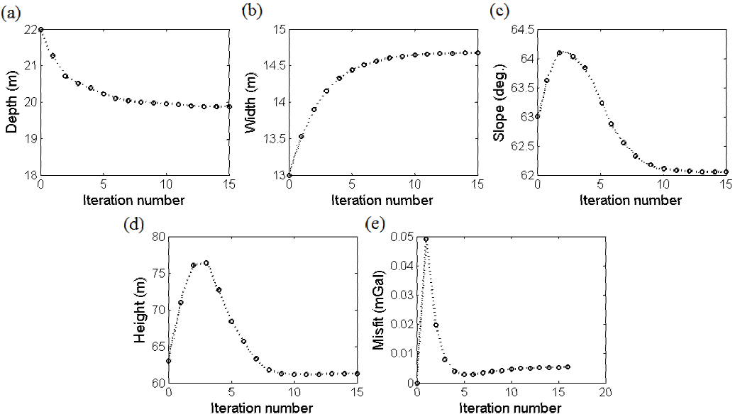
Figure 11 Variations of a) depth b) width c) dip d) height and e) misfit function versus iteration number for 10% noise corrupted synthetic gravity data shown in figure 5.
Figure 12(a) shows the inverted gravity anomaly calculated from the inverted model parameters which is shown in Figure 12(b). The theoretical parameters and inferred values for the noise corrupted synthetic gravity data have been summarized in Table 2.
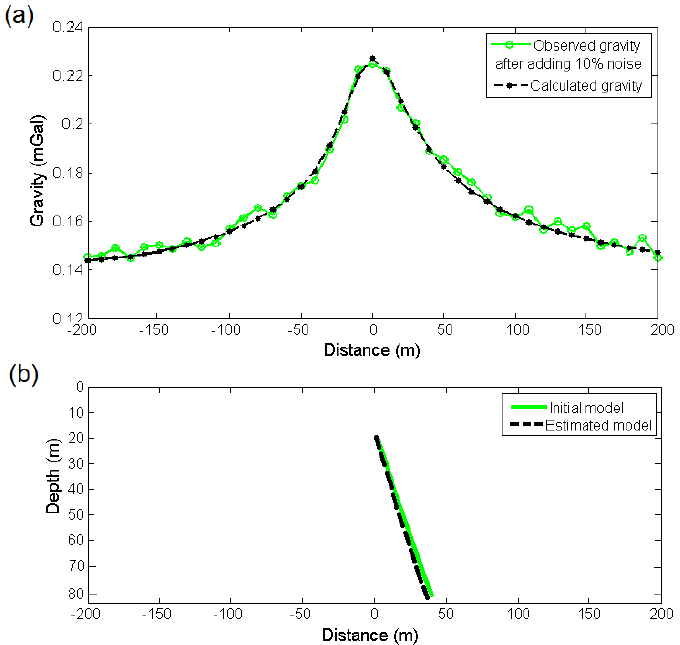
Figure 12 a) The observed gravity anomaly with a added random noise of 10% and calculated gravity anomaly along a profile due to b) the initial (z=20 m, w=15 m, α=60 degree and H= 60 m) and estimated (z=19.9 m, w=14.7 m, α =62.08 degree and H= 61.5 m) models with a density contrast of 1000 kg/m3
Table 2 Numerical results obtained from the Marquardt inversion of the noise corrupted synthetic gravity data
| Parameter | Depth (m) | Width (m) | Dip α (degree) | Height (m) |
|---|---|---|---|---|
| Initial | 20 | 15 | 60 | 60 |
| Assumed | 22 | 13 | 63 | 63 |
| Estimated | 19.9 | 14.7 | 62.08 | 61.5 |
| Error % | 0.1 | 2 | 3.67 | 2.5 |
| Iteration | 15 | |||
| Misfit (mGal) | 0.0053 | |||
To investigate the solutions constancy and performance of the Marquardt inversion, two different initial and assumed dyke models were assumed to analyze the gravity anomalies related to them with and without a random noise of 10% (Table 3 and 4). The estimated structural parameters are almost corresponde to the initial ones.
Table 3 Inverted parameters from analysis of free-noise gravity anomalies for different models
| Parameter | With 10% random noise | |||||||
|---|---|---|---|---|---|---|---|---|
| Model 1 | Model 2 | |||||||
| Depth (m) | Dip (deg) | Width (m) | Height (m) | Depth (m) | Dip (deg) | Width (m) | Height (m) | |
| Initial | 25 | 50 | 12 | 45 | 40 | 110 | 20 | 65 |
| Assumed | 30 | 60 | 16 | 40 | 32 | 100 | 14 | 58 |
| Estimated | 25.01 | 49.97 | 11.99 | 45.02 | 39.97 | 110.1 | 20.02 | 65.03 |
| Error % | 0.04 | 0.06 | 0.083 | 0.044 | 0.075 | 0.091 | 0.1 | 0.046 |
| Misfit (nT) | 0.00000072 | 0.0000094 | ||||||
| Lambda λ | 2.4×10⁻¹² | 5.7×10⁻²³ | ||||||
| Iteration | 12 | 18 | ||||||
Table 4 Inverted parameters from analysis of 10% noise-corrupted gravity anomalies for different models
| Parameter | With 10% random noise | |||||||
|---|---|---|---|---|---|---|---|---|
| Model 1 | Model 2 | |||||||
| Depth (m) | Dip (deg) | Width (m) | Height (m) | Depth (m) | Dip (deg) | Width (m) | Height (m) | |
| Initial | 25 | 50 | 12 | 45 | 40 | 110 | 20 | 65 |
| Assumed | 30 | 60 | 16 | 40 | 32 | 100 | 14 | 58 |
| Estimated | 25.2 | 50.3 | 11.85 | 45.13 | 38.84 | 112.6 | 19.6 | 66.8 |
| Error % | 0.04 | 0.06 | 0.083 | 0.044 | 2.9 | 2.36 | 2 | 2.77 |
| Misfit (nT) | 0.000086 | 0.078 | ||||||
| Lambda λ | 7.1×10⁻¹⁸ | 32.8 | ||||||
| Iteration | 19 | 23 | ||||||
Real gravity analysis
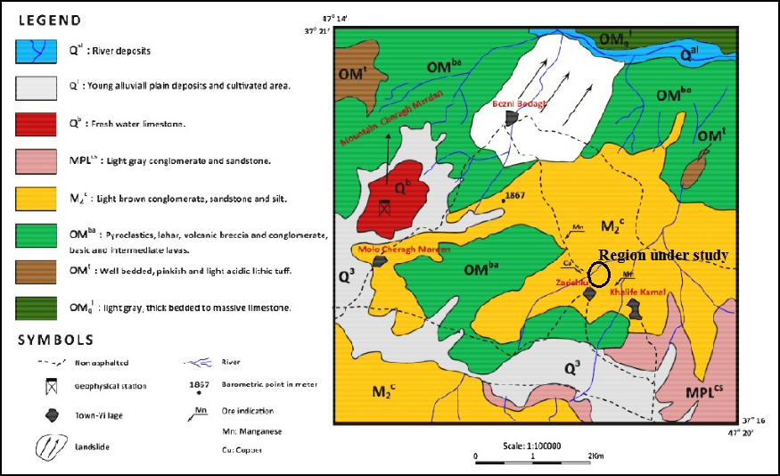
Real gravity data are from the Zereshlu Mining Camp, situated in the west of Mianeh, East Azerbaijan Province, Iran. The main mineral in this area is Manganese which exists mostly in the form of vein deposit or sheet-like structure with the origin of the hydrothermal.
Figure 13 exhibits the geological map of the region around the Zereshlu mine. The gravity measurement region is indicated by a black circle. The predominant rocks in the region under investigation are the conglomerate, sandstone and silt. As well as, in this region there are the layers of the basalt, andesite and altered andesite with ferrous oxide. These rocks are considered as the host rocks of the manganese dioxide mineral which is thought to have filled the major faults and fractures. The net density of manganese dioxide is 4.75 gr/cm3 and the average density of the basalt and andesite are about 2.9 gr/cm3 and 2.6 gr/cm3, respectively. When the ferrous oxide and manganese dioxide are dispersed in the basalt and andesite, therefore, the density of the host rock and that of the target, can consider between 3.2 gr/cm3 to 3.5 gr/cm3. The background density of the study area is about 2.6 gr/cm3, thus the density contrast between the body causative of gravity anomalies, i.e. the host rocks, and background domain range between 0.6 gr/cm3 to 0.9 gr/cm3 (on average 0.75 gr/cm3).
The gravity survey district in zone 38, stretches the UTM coordinate from 704410 m to 704555 m East and from 4130820 m to 4131000 m North. The Bouguer gravity anomaly map of the study area is shown in Figure 14. After removing the effect of regional gravity field from the Bouguer gravity anomaly, the residual gravity anomalies map is achieved (Figure 15). The linear gravity anomalies whose values are positive indicate the sources that are rich in the Manganese. The gravity sampling was performed at 33 points with an interval of1.03 m along the 34 m profile AA', which runs across the dyke-like structure in the W-E direction (Figure 15). We apply the variations of the residual gravity field at the observed points over the profile AA' for reconstructing the buried structure.
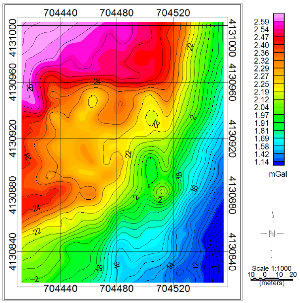
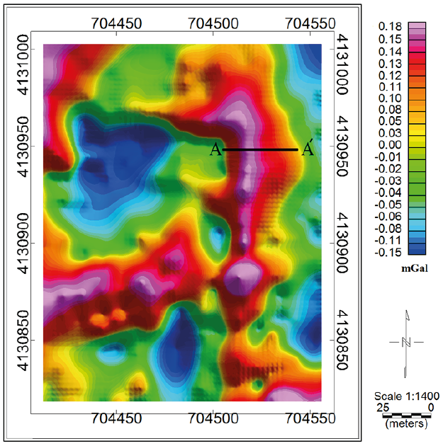
Figure 15 The residual gravity anomalies map of the study district. The profile AA' is specified in W-E direction.
For inverting the real gravity data (Figure 17a) using the damped SVD technique, the underground study domain was divided into 33 × 17=561 rectangular prisms with respective dimensions of 1.5 × 2.5 m. Figure 16 shows the density distribution that resulted from the linear inversion. The blocks whose densities are between 3.2 gr.cm3 to 3.5 gr/cm3 foreshow the manganese deposit body.
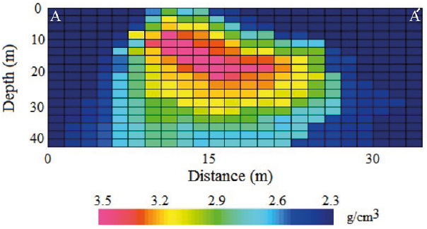
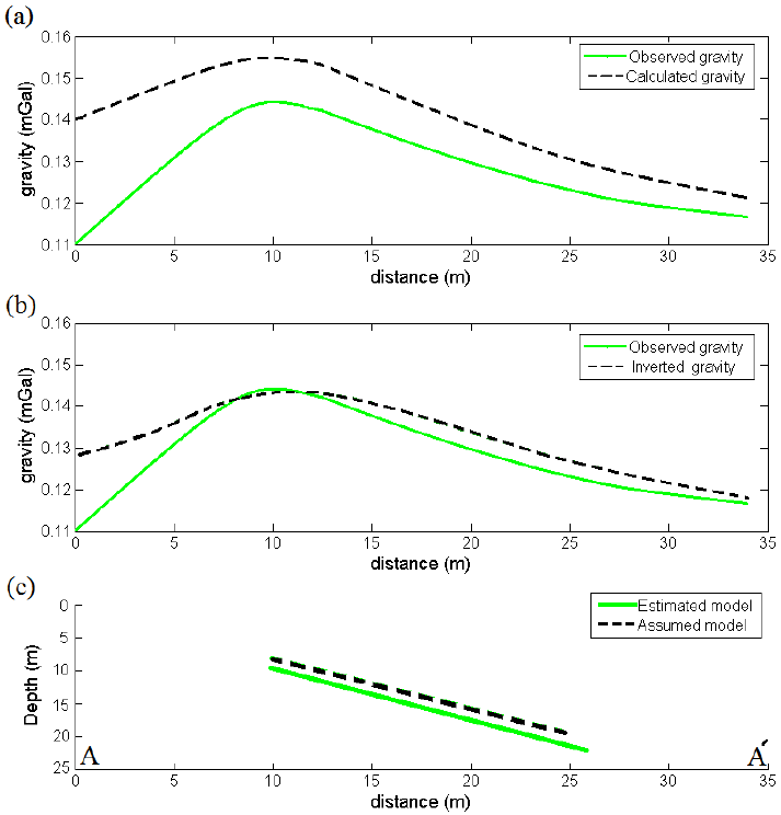
Figure 17 A) The observed gravity along the profile AA' and calculated gravity due to the assumed model, b) Inferred gravity from estimated structure, c) The assumed model and estimated model obtained by the Marquardt inversion.
Inversion of the observed gravity data (Figure 17a) using the Marquardt inversion technique, we assume an initial model whose parameters values are given as z=8 m, w=17 m, α=38 degree and H=19 m (Figure 17c). The calculated gravity due to the assumed model is shown in Figure 17(a). Moreover, the assigned values for misfit (J), iteration and damping factor (λ) are 0.0005 nmGal, 50 and 15, respectively.
The changes of each parameter and misfit against the iteration number during the inversion process are shown in Figures 18(a) to 18(d). The algorithm performed 10 iterations, before it ceased, since at the end of this iteration number, the damping factor reached a value greater than the predefined value (see Table 5).
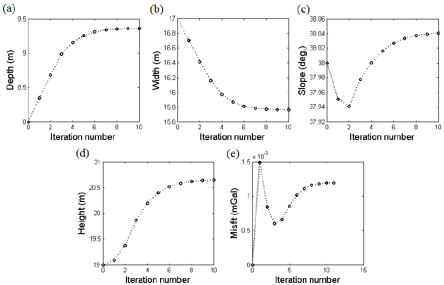
Figure 18 The variations of a) depth b) width c) dip d) height and e) misfit function versus iteration number for the real gravity data.
Table 5 The initial parameters values and final parameters values from interpretation of the real gravity data
| Parameter | Depth (m) | Width (m) | Dip α (deg) | Height (m) |
|---|---|---|---|---|
| Assumed | 8 | 17 | 38 | 19 |
| Estimated | 9.4 | 15.8 | 38.04 | 20.3 |
| Final Misfit (mGal) | 0.00122 | |||
| Final Lambda λ | 24.68 | |||
| Iteration | 10 | |||
The misfit function variations versus the iteration number (Figure 18e) show a fast decrease from its first value of 0.00015 mGal to its value at the 3th iteration and then increase continually until 10th iteration whose value is 0.000127 mGal. The depth and height parameters increase steadily from its initial value to their final values at the 10th iteration whose values are 9.4 m and 20.3 m, respectively (Figures 18a and 18d). The width parameter decreases significantly until 6th iteration and then gradually achieved 15.8 m at the 10th iteration (Figure 18b). The dip parameter reduces from its initial value to its value at the 3th iteration and then increased rapidly until 10th iteration where it was obtained a value of 38.04 degree towards the east (Figure 18c). The resulted tabular model is delineated in Figure 17(c). The gravity response estimated from the inferred parameters for the dyke-like structure (Figure 17c) is shown in Figure 17(b). The inverted structural parameters are given in Table 5.
Discussion and conclusions
In this paper, we have introduced two inverse modeling methods, based on the damped singular value decomposition (DSVD) as a linear inversion and the Marquardt optimization algorithm as a nonlinear inversion. The Marquardt optimization algorithm has been developed for interpreting the gravity data due to a dyke-like structure. The validation and performance of the both approaches were evaluated using the theoretical gravity data, with and without random noise. The inverted models obtained from the analysis of the synthetic gravity data via the both methods are exactly similar to the initial ones. The Marquardt inversion shows an acceptable convergence for the various assumed parameters. We employed the both methods for inverting the real gravity data due to a near surface sheet-like structure from Iran. In the resulted density distribution by the damped SVD inversion, the adjacent blocks with a density bigger than 3.2 gr/cm3, demonstrate the geometry of the Manganese ore deposit. Considering to inverted density distribution, the depth to the top and bottom of the simulated structure with a direction of NW-SE, are about 7.5 m and 25 m, respectively. Moreover, the average amount of width and extension of the interpreted structure are given about 15 m and 22 m, respectively. As the distribution density resulted from the damped SVD inversion demonstrate a subsurface dyke-like structure, therefore, we can apply the Marquardt optimization algorithm for analyzing the gravity data. The inferred parameters using the Marquardt inversion of the real gravity data demonstrate a dyke-like structure with a width of 15.8 m, a dip of 38.04 degree and a height (extension) of 20.3 m where the depth to the top and bottom are 9.4 m and 21.9 m, respectively.
The comparison of the parameters values of the inverted structures from the damped SVD inversion and the Marquardt optimization method shows a close affinity between them. Therefore, using from the both inversion methods can be a helpful and advantageous strategy in the accurate interpretation of the gravity data.

