


 nueva página del texto (beta)
 Inglés (pdf)
 Artículo en XML
 Referencias del artículo
 Enviar artículo por email
 Citado por SciELO
  Similares en
SciELO
Similares en
SciELO 
 Permalink
Introduction
An artificial neural network (ANN) is an effective tool that has been used to solve a great variety of engineering problems due to its flexibility to cope highly nonlinear problems. It is worth mentioning that ANN models as any other prediction technique have advantages and disadvantages (Pande and Shin, 2004). Some advantages of using ANN models include the storage information of the ANN with multidimensional inputs, the prediction of multiple outputs with a single ANN model, the ability to work with incomplete knowledge and machine learning. Perhaps two of the major draw-backs of ANN models are the loss of transparency and the unexpected behavior of the ANN model that may produce erroneous results.
The employ of ANNs in seismic engineering is vast, for example, García et al. (2007), used ANNs to estimate peak ground accelerations (PGA) for Mexican subduction earthquakes. Hong et al. (2012), employed 39 California earthquakes to predict pseudospectral accelerations (SA) and PGA. More recently, Pozos-Estrada et al. (2014) developed ANNs models to predict PGA and SA for Mexican inslab and interplate earthquakes. They showed that the predicted PGA and SA values by the trained ANN models, in general, follow a similar trend to those predicted by ground motion prediction equations (GMPEs). ANNs have also been used to estimate strong ground motion duration (SGMD) of earthquakes. Alcántara et al. (2014), developed ANNs to predict SGMD by using information compiled from the Mexican states of Puebla and Oaxaca. The prediction of SGMD has also been applied to other tectonic regions, for example Arjun and Kumar (2011), used ANN models to estimate the SGMD by using Japanese earthquake records, and more recently, Yaghmaei-Sabegh (2018), used a general regression neural network to estimate earthquake ground-motion duration recorded at the Iranian plateau.
The study of SGMD to estimate the structural damage has also been carried out by several researchers (Housner et al. 1952; Salmon et al., 1992; Bommer and Martínez, 1999; Strasser and Bommer 2009; and Lindt and Goh, 2004). The general agreement among these studies is that the structural damage not only depend on the maximum intensity or frequency content of the ground motion, but also on the SGMD. For the estimation of the seismic-induced structural response, the amplitude and frequency content of the ground motions are of paramount importance; however, if the cumulative structural damage or structural degradation of systems with hysteretic behavior is of interest, SGMD should be integrated as design parameter (Reinoso and Ordaz, 2001). More recently, Bhargavi and Raghukanth (2019), carried out a statistical analysis of several ground motion parameters, including SGMD, to rate damage potential of ground motion records.
The main objective of this study is to develop ANN models to estimate SGMD of interplate and inslab ground motion records of Mexican earthquakes from a broad network of stations. Ground motion records from 1985 up to 2017 are employed. Multilayer perceptron ANN models with back-propagation training were considered. The input parameters considered in the development of the ANN models include the moment magnitude (Mw), closest distance to the fault (RC), focal depth (H), the vibration period of the soil (T), the seismic moment (M0), as well as the strike (φ), dip (δ) and rake (λ) angles. The principal component method is used to carry out a dimensionality reduction of the input parameters to evaluate the ability of ANN models with different number of input parameters to predict the SGMD. The predicted SGMD values by the trained ANN models are compared with those estimated with empirical equations for comparison purposes.
Strong Ground Motion Database and SGMD Calculation
The strong ground motion database employed integrates information from different networks. A total of 3153 strong ground motion records, each one with two horizontal components from 71 earthquakes were used to develop the ANN models. Table 1 and 2 summarize the interplate and inslab seismic events considered, respectively. The database for interplate includes 50 events with Mw from 5.0 to 8.1, while de database for intermediate-depth normal-faulting inslab events considers 21 with Mw within 5.1 and 7.1. It is noted that the seismic event occurred on September 7, 2017 was not included in the inslab database since it did not cause important damage in Mexico City (Pozos-Estrada et al., 2019) and because the peak ground acceleration registered in Mexico City at lake-bed was below 4 Gal, which was the threshold recommended by Reinoso and Ordaz (2001) as selection criterion of records to calculate SGMD. However, the inslab event occurred on September 19, 2017, which was, together with the interplate event occurred on September 19, 1985, one of the deadliest for Mexico City (Singh et al., 2018, Franke et al., 2019) was included. A map showing the epicenters and recording stations considered is presented in Figure 1. Also in Figure 1, the geotechnical zones (i.e., firm, transition and lakebed) according to the Mexico City design code (2017) are presented. It is worth mentioning that the Mexico City design code (2017) includes rock in the firm soil zone. Figure 2 presents the distribution of Mw, H and M0 with respect to RC for the seismic events used.
Table 1 Interplate events used in training the ANN models
| Event No. | No. of Rec. | Date (dd/mm/yy) | Mw | Lat.°N | Long °W | H (km) | Institution* |
|---|---|---|---|---|---|---|---|
| 1 | 9 | 19/09/85 | 8.1 | 18.081 | 102.94 | 15 | CFE-GIEC, II**, IG** |
| 2 | 22 | 21/09/85 | 7.6 | 18.021 | 101.48 | 15 | CFE-GIEC, II**, IG** |
| 3 | 8 | 29/10/85 | 5.4 | 17.583 | 102.64 | 20.3 | CFE-GIEC, II**, IG** |
| 4 | 19 | 30/04/86 | 7.0 | 18.024 | 103.06 | 20 | CFE-GIEC, II**, IG** |
| 5 | 8 | 05/05/86 | 5.5 | 17.765 | 102.80 | 19.9 | CFE, II**, IG** |
| 6 | 60 | 08/02/88 | 5.8 | 17.494 | 101.16 | 19.2 | CFE, CIRES, FICA, II**, IG** |
| 7 | 114 | 25/04/89 | 6.9 | 16.603 | 99.4 | 19 | CFE, CIRES, FICA, II**, IG** |
| 8 | 112 | 31/05/90 | 5.9 | 17.106 | 100.89 | 16 | CENAPRED, CIRES, FICA, GIEC, II**, IG** |
| 9 | 50 | 01/04/91 | 5.4 | 16.044 | 98.39 | 25.6 | CENAPRED, CIRES, FICA, II**, IG** |
| 10 | 22 | 31/03/92 | 5.1 | 17.233 | 101.30 | 11 | CENAPRED, CFE, FICA, II**, IG** |
| 11 | 74 | 15/05/93 | 5.5 | 16.47 | 98.72 | 15 | CIRES, II**, IG** |
| 12 | 200 | 24/10/93 | 6.6 | 16.54 | 98.98 | 5 | CENAPRED, RIIS, GIEC, CIRES, II**, IG** |
| 13 | 6 | 13/11/93 | 5.4 | 15.63 | 99.02 | 15 | CIRES, II**, IG** |
| 14 | 240 | 10/12/94 | 6.3 | 18.02 | 101.56 | 20 | CENAPRED, RIIS, GIEC, CIRES, II**, IG** |
| 15 | 149 | 14/09/95 | 7.3 | 16.31 | 98.88 | 22 | CENAPRED, CIRES, RIIS, II**, IG** |
| 16 | 138 | 09/10/95 | 7.3 | 18.74 | 104.67 | 5 | CENAPRED, CIRES, GIEC, RIIS, II*, IG** |
| 17 | 55 | 12/10/95 | 5.5 | 19.04 | 103.70 | 11 | CENAPRED, CIRES, IG** |
| 18 | 62 | 25/02/96 | 6.9 | 15.83 | 98.25 | 5 | CENAPRED, CIRES, II**, IG** |
| 19 | 186 | 15/07/96 | 6.5 | 17.45 | 101.16 | 20 | CENAPRED, CIRES, GIEC, RIIS, II**, IG** |
| 20 | 196 | 11/01/97 | 6.9 | 17.9 | 103.04 | 16 | CPRED, CIRES, GIEC, RIIS, II**, IG** |
| 21 | 18 | 21/01/97 | 5.4 | 16.44 | 98.15 | 18 | CENAPRED, CIRES, II**, IG** |
| 22 | 32 | 19/07/97 | 6.3 | 15.86 | 98.35 | 5 | CENAPRED, CIRES, II**, IG** |
| 23 | 18 | 16/12/97 | 5.9 | 15.7 | 99.04 | 16 | CIRES, II*, IG** |
| 24 | 22 | 22/12/97 | 5.0 | 17.14 | 101.24 | 5 | CENAPRED, CIRES, II**, IG** |
| 25 | 82 | 03/02/98 | 6.2 | 15.69 | 96.37 | 33 | CENAPRED, CIRES, II**, IG** |
| 26 | 12 | 05/07/98 | 5.0 | 16.83 | 100.12 | 5 | CENAPRED, II**, IG** |
| 27 | 246 | 30/09/99 | 7.5 | 15.95 | 97.03 | 16 | CENAPRED, CIRES, II**, IG**, RIIS |
| 28 | 149 | 09/08/00 | 6.1 | 17.99 | 102.66 | 16 | CIRES, II**, IG** |
| 29 | 48 | 08/10/01 | 5.4 | 16.94 | 100.14 | 10 | II**, IG** |
| 30 | 68 | 18/04/02 | 5.4 | 16.77 | 101.12 | 22 | CIRES, II*, IG** |
| 31 | 32 | 22/01/03 | 7.5 | 18.6 | 104.22 | 9 | II**, IG** |
| 32 | 67 | 01/01/04 | 5.6 | 17.34 | 101.42 | 6 | CIRES, II**, IG** |
| 33¥ | 186 | 13/04/07 | 6.3 | 17.09 | 100.44 | 41 | CIRES, II**, IG** |
| 34 | 46 | 06/11/07 | 5.6 | 17.08 | 100.14 | 9 | II**, IG** |
| 35 | 74 | 27/04/09 | 5.7 | 16.9 | 99.58 | 7 | CIRES, II, IG |
| 36 | 48 | 09/02/10 | 5.8 | 15.9 | 96.86 | 37 | II, IG |
| 37 | 124 | 30/06/10 | 6.0 | 16.22 | 98.03 | 8 | CIRES, II, IG |
| 38 | 176 | 20/03/12 | 7.4 | 16.251 | 98.521 | 16 | CIRES, II, UAP, IG |
| 39 | 162 | 02/04/12 | 6.0 | 16.27 | 98.47 | 10 | CIRES, II, UAP, IG |
| 40 | 17 | 11/04/12 | 6.4 | 17.9 | 103.06 | 16 | CIRES, II, IG |
| 41 | 48 | 22/09/12 | 5.4 | 16.23 | 98.30 | 10 | CIRES, II |
| 42 | 36 | 22/04/13 | 5.8 | 17.87 | 102.19 | 10 | II |
| 43 | 60 | 21/08/13 | 6.0 | 16.79 | 99.56 | 16 | II |
| 44 | 193 | 18/04/14 | 7.2 | 17.18 | 101.19 | 10 | CIRES, II |
| 45 | 190 | 08/05/14 | 6.4 | 17.11 | 100.87 | 17 | CIRES, II |
| 46 | 50 | 10/05/14 | 6.1 | 17.16 | 100.95 | 12 | CIRES, II |
| 47 | 46 | 11/10/14 | 5.6 | 15.97 | 95.61 | 10 | II |
| 48 | 58 | 23/11/15 | 5.8 | 16.86 | 98.94 | 10 | II |
| 49 | 78 | 08/05/16 | 6.0 | 16.25 | 97.98 | 35 | II |
| 50 | 38 | 27/06/16 | 5.7 | 16.2 | 97.93 | 20 | II |
Notes: * II: Institute of Engineering from UNAM (http://aplicaciones.iingen.unam.mx/AcelerogramasRSM/Consultas/Filtro.aspx); IG: Institute of Geophysics from UNAM (http://www2.ssn.unam.mx:8080/catalogo/); CENAPRED: National Center for Disaster Prevention (http://geografica.cenapred.unam.mx:8080/reporteSismosGobMX/BuscarAcelerograma); CIRES: Instrumentation and Seismic Record Center (http://www.cires.org.mx/racm_historico_es.php); RIIS: Interuniversity Network of Seismic Instrumentation; FICA: ICA Foundation; GIEC: Experimental Engineering and Control Management; UAP: Autonomous University of Puebla. ** Some of the records used were compiled by García (2005) and García et al. (2006). ¥Interplate event according to Franco et al., (2007).
Table 2 Inslab events used in training the ANN models.
| Event No. | No. of Rec. | Date (dd/ mm/yy) | Mw | Lat. °N | Long. °W | H (km) | Institution* |
|---|---|---|---|---|---|---|---|
| 1¥ | 10 | 05/08/93 | 5.1 | 17.08 | 98.53 | 32 | CENAPRED, II**, IG** |
| 2¥ | 16 | 23/02/94 | 5.4 | 17.82 | 97.30 | 5 | II**, IG**, CENAPRED |
| 3¥ | 166 | 23/05/94 | 5.6 | 18.03 | 100.57 | 23 | CENAPRED, CIRES, RIIS, II**, IG** |
| 4¥ | 130 | 10/12/94 | 6.4 | 18.02 | 101.56 | 20 | CIRES, II**, IG** |
| 5¥ | 124 | 11/01/97 | 6.9 | 17.9 | 103.00 | 16 | CIRES, II**, IG** |
| 6¥ | 4 | 03/04/97 | 5.1 | 17.98 | 98.33 | 30 | II**, IG** |
| 7 | 144 | 22/05/97 | 6.0 | 18.41 | 101.81 | 59 | CENAPRED, CIRES, RIIS, II**, IG** |
| 8 | 38 | 20/04/98 | 5.1 | 18.37 | 101.21 | 66 | CENAPRED, CIRES, RIIS, II**, IG** |
| 9 | 254 | 15/06/99 | 6.5 | 18.18 | 97.51 | 69 | CENAPRED, CIRES, RIIS, II**, IG** |
| 10 | 172 | 21/06/99 | 5.8 | 17.99 | 101.72 | 54 | CENAPRED, CIRES, II**, IG** |
| 11 | 202 | 13/04/07 | 6.3 | 17.37 | 100.14 | 42 | CIRES, II**, IG** |
| 12 | 88 | 12/02/08 | 6.5 | 16.35 | 94.51 | 87 | CIRES, II**, IG** |
| 13 | 52 | 22/05/09 | 5.7 | 18.13 | 98.44 | 45 | II**, IG** |
| 14 | 40 | 21/07/00 | 5.4 | 18.09 | 98.97 | 48 | II**, IG** |
| 15 | 80 | 07/04/11 | 6.7 | 17.2 | 94.34 | 167 | CIRES, II |
| 16 | 210 | 11/12/11 | 6.5 | 17.89 | 99.84 | 58 | CIRES, II, UAP |
| 18 | 156 | 15/11/12 | 6.1 | 18.17 | 100.52 | 40 | CIRES, II, UAP |
| 19 | 50 | 29/07/14 | 6.4 | 17.7 | 95.63 | 117 | CIRES, II |
| 20 | 148 | 19/09/17 | 7.1 | 18.4 | 98.72 | 57 | CIRES, II, UAP |
| 21 | 68 | 23/09/17 | 6.1 | 16.48 | 94.90 | 75 | CIRES |
Notes: * II: Institute of Engineering from UNAM (http://aplicaciones.iingen.unam.mx/AcelerogramasRSM/Consultas/Filtro.aspx); IG: Institute of Geophysics from UNAM (http://www2.ssn.unam.mx:8080/catalogo/); CENAPRED: National Center for Disaster Prevention (http://geografica.cenapred.unam.mx:8080/reporteSismosGobMX/BuscarAcelerograma); CIRES: Instrumentation and Seismic Record Center (http://www.cires.org.mx/racm_historico_es.php; RIIS: Interuniversity Network of Seismic Instrumentation; FICA: ICA Foundation; GIEC: Experimental Engineering and Control Management; UAP: Autonomous University of Puebla. **Some of the records used were compiled by García (2005) and García et al., (2006). ¥Cortical events Lowry et al., (2001).


Figure 2 Distribution of Mw, H and M0 with respect to RC: (a), (b) and (c) for interplate events; (d), (e) and (f) for inslab events.
For the analyses, only two type of soils were considered (soft and firm soil). The transition zone was included in the classification of soft soil on the basis that the dominant period of the soil at such zone is greater than 0.5 s, which is the limiting value used in the Mexican design code to separate firm soil from the rest, and that no evidence that duration is affected by amplification effects on strong ground motion (Singh and Ordaz, 1993). It is worth mentioning that the soft soil of Mexico City consists of lacustrine deposits with saturated clays and sand lenses, the transition soil is composed by alluvial deposits and the firm soil consists of basaltic and andesitic lava, ashes and epiclastic deposits (Marsal and Mazari, 1959; Flores-Estrella et al., 2007). The firm soil of Mexico City can be classified as class B according to NEHRP Recommended provisions for seismic regulations for new buildings and other structures (2004).
The total number of records from interplate and inslab events were organized into three groups. The first group corresponds to seismic records registered at soft soil of Mexico City (SS-MC), the second group corresponds to seismic records registered at firm soil of Mexico City (FS-MC), and the third group includes the rest of records registered outside Mexico City at firm soil (i.e., rock) (FS-M). For the development of the ANN models and the empirical equations, a database with all horizontal components of motion without combining them was considered. Figure 3 presents a plot with the percentage of seismic records from interplate and inslab earthquakes used in each group as well as the type of soil. It is observed from Figure 3 that the distribution of records per group is similar between the interplate and inslab earthquakes, and that the records for sites with soft soil in Mexico City have the greatest percentage.

Data Processing
A program was developed in MATLAB (2019), to build a database of seismic records for each type of earthquake. The information considered for each record included the name of the file, station name, station coordinates, magnitude of the event, epicentral coordinates, date and hour of the seismic event, orientation of each sensor channel, peak ground acceleration and maximum seudoacceleration for each component for the soil period, strong ground motion duration and the acceleration values for each component. Bad quality records were discarded. A baseline correction of all the time histories of the records was carried out. Further, for events registered at firm soil (including rock) with Mw >6.5, a high-pass filter with a cut-off frequency of 0.05 Hz was used, for the rest events, a high-pass corner frequency 0.1 Hz was employed. This processing criterion was guided by the work of García et al. (2005) and García (2006). For events registered at soft soil, a band-pass filter with corner frequencies from 0.1 to 10 Hz was employed (Jaimes et al., 2015).
SGMD Calculated from the Processed Data
The study of the SGMD has been carried out by several researchers in the past (Trifunac and Brady et al., 1975; Trifunac and Westermo et al., 1982). In this study the SGMD was calculated based on the accumulation of energy along time of the strong ground motion records. Arias intensity (Arias, 1970) has been widely used to relate the SGMD with the acceleration time history energy, although it has also been used to study the damage patterns and principal direction of seismic excitations (Arias, 1996; Hong and Goda, 2007; and Hong et al., 2009). In this study the SGMD is assessed based on the Arias intensity, defined as
where a(t) is the acceleration time history, t 0 is the total duration of the strong ground motion and g is the acceleration due to gravity. Several procedures have been reported in the literature to determine the SGMD (Bommer and Martínez, 1999), based on lower and upper bounds of duration related to I A . According to Reinoso and Ordaz (2001), SGMD for Mexican earthquakes can be obtained based on the duration of the strong ground motion between 2.5 and 97.5% of I A , which is useful for engineering problems. These limits are adopted in the present study, since the records employed in the databases also include most of those used in Reinoso and Ordaz (2001).
Artificial Neural Network Modeling and Training
The ANN architecture with multiple hidden layers and neurons used in this study is shown in Figure 4, where three main layers can be identified: input, hidden and output layer. The flow of information starts from the input layer, this information is weighted to optimize the mapping between the input and the hidden layer(s), and finally transferred it into output value(s). The information transferred from the hidden layer(s) to the output layer is affected by biases that modified the output of the neuron. If an ANN model with a single output neuron and two hidden layers is considered, the mathematical expressions that relate the output neuron in the output layer with the neurons in input and hidden layers are given by,
where y output is the value of the output neuron, O IL-HL1 is the outcome obtained when the information given in the input layer has passed through the first hidden layer, O HL1-HL2 is the outcome obtained when the information from the first hidden layer has passed through the second hidden layer, m is the total number of neurons in the hidden layers, n is the total number of neurons in the input layer, f 1 ( ), f 2 ( ) and f 3 ( ) are activation functions between the input and the first hidden layer, the first and the second hidden layer and between the second hidden layer and the output layer, respectively; [w 1 ] i,j , [w 2 ] j,k and [w 3 ] k,1 are the weights that map the information between the input and the first hidden layer, between the first and second hidden layer and between the second hidden layer and output layer, respectively; (φ1) j , (φ2) k and (φ3) 1 are the biases associated with the hidden and output layers and x i is the i-th neuron in the input layer.

The optimization of the weights and biases of the ANN model is carried out during the training process. Although a variety of algorithms is available in the literature (Swingler, 1996; Principe and Euliano, 1999; and Haykin, 1999), the back-propagation algorithm (Rumelhart et al., 1986) is one of the most popular. The back-propagation algorithm employs a predefined error function, which is minimized to evaluate the weights and biases. The back-propagation algorithm is adopted in the present study to train the ANN models. Aside from the back-propagation algorithm, in the last decade the constant improvement of Machine Learning techniques has allowed the development of deep learning that employs the deep neural network. The use of deep neural networks has gained much attention due to their ability to solve complex problems. The use of deep neural networks is outside of the scope of the present study.
Estimation of Strong Ground Motion Duration Using Ann
Application of Principal Component Analysis to Identify the Inputs of the ANNs Models
Dimensionality reduction methods have been widely used to reduce the number of input parameters to develop ANN models (Yuce et al., 2014). One of the classical dimensionality reduction methods is the principal component analysis (PCA), which transforms a set of observations of correlated variables into a set of principal components, which are linearly uncorrelated. Based on the identified principal components, the amount of total variance contributed by each component is assed to select a reduced number of principal components which cumulative variance is within predefined acceptable values. Once a reduced number of principal components is selected, the relative importance of each input parameter to a particular component is evaluated by using correlation coefficients that relate the reduced set of principal components and input parameters. The reduced number of input parameters is selected based on predefined thresholds of correlation coefficients.
To illustrate the use of PCA in the dimensionality reduction of the input neurons for the development of the ANN models, we use the data for inslab events for firm soil for places outside Mexico. To proceed with the calculation of the principal components, the correlation coefficient matrix between the input variables is given in Table 3.
Table 3 Correlation coefficient matrix for input variables for inslab events for firm soil for places outside Mexico.
| RC | Mw | T | H | M0 | φ | δ | λ | |
|---|---|---|---|---|---|---|---|---|
| RC | 1 | 0.220 | 0.347 | 0.242 | 0.124 | 0.215 | -0.028 | -0.101 |
| Mw | 0.220 | 1 | 0.087 | 0.397 | 0.659 | 0.123 | 0.384 | -0.002 |
| T | 0.347 | 0.087 | 1 | 0.119 | 0.033 | 0.099 | -0.056 | -0.015 |
| H | 0.242 | 0.397 | 0.119 | 1 | 0.046 | 0.457 | 0.200 | -0.284 |
| M0 | 0.124 | 0.659 | 0.033 | 0.046 | 1 | 0.160 | 0.124 | -0.210 |
| φ | 0.215 | 0.123 | 0.099 | 0.457 | 0.160 | 1 | -0.308 | -0.053 |
| δ | -0.028 | 0.384 | -0.056 | 0.200 | 0.124 | -0.308 | 1 | 0.326 |
| λ | -0.101 | -0.002 | -0.015 | -0.284 | -0.210 | -0.053 | 0.326 | 1 |
The correlation coefficient matrix is then decomposed by using the singular value decomposition to calculate the amount of total variance contributed by each principal component. Table 4 summarizes the percentage of variance associated with each principal component and its corresponding eigenvalue.
Table 4 Percentage of variance associated with each principal component and its corresponding eigenvalue.
| Principal component | 1 | 2 | 3 | 4 | 5 | 6 | 7 | 8 |
|---|---|---|---|---|---|---|---|---|
| Eigenvalue | 2.24 | 1.64 | 1.19 | 1.03 | 0.87 | 0.63 | 0.29 | 0.11 |
| Variance (%) | 27.99 | 20.46 | 14.84 | 12.90 | 10.89 | 7.82 | 3.66 | 1.41 |
| Cumulative variance (%) | 27.99 | 48.46 | 63.30 | 76.20 | 87.10 | 94.92 | 98.59 | 100 |
It is noted that there are different criteria to select the reduced number of principal components. According to Lovric (2011), the reduced number of principal components can be selected when they account for a cumulative variance within 70 to 90%. A simpler criterion, which is adopted in this study, is to select those principal components whose eigenvalues are greater than one. Based on the afore-mentioned criterion, from Table 4, the reduced number of principal components is equal to 4.
By using the first 4 principal components, the correlation coefficients that relate the reduced set of principal components and input parameters is presented in Table 5.
Table 5 Correlation coefficients that relate the reduced set of principal components and input parameters.
| Input parameter | 1 | 2 | 3 | 4 |
|---|---|---|---|---|
| RC | 0.531 | -0.261 | 0.466 | -0.255 |
| Mw | 0.784 | 0.476 | -0.114 | -0.069 |
| T | 0.321 | -0.254 | 0.638 | -0.414 |
| H | 0.688 | -0.153 | 0.046 | 0.582 |
| M0 | 0.635 | 0.289 | -0.437 | -0.424 |
| φ | 0.495 | -0.511 | -0.017 | 0.420 |
| δ | 0.193 | 0.823 | 0.242 | 0.225 |
| λ | -0.284 | 0.483 | 0.546 | 0.211 |
It is observed in Table 5 that there are considerable variation in the correlation coefficients. To identify the reduced input parameters, we use two thresholds of correlation coefficients (Moore et al., 2013), the first one equals 0.7 and the second one equals 0.55. It is noted that strong relation between variables is associated with correlation coefficients greater than 0.7, while moderate relation is associated with correlation coefficients greater than 0.55. Table 6 presents the reduced number of input parameters when the correlation thresholds are adopted. Also in Table 6, the reduced number of input parameters for the rest of the database are summarized. It is observed from Table 6 that the number of input parameters with strong correlation for interplate events ranges from 2 to 3, while for inslab it varies from 2 to 6. For the input parameters with strong correlation, the greater number of input parameters are related to the SS-MC case. If moderate correlation is considered, the number of input parameters is within 6 to 7 and 5 to 7 for interplate and inslab events, respectively. Based on the PCA results, ANN models are developed by using the identified input parameters based on the type of relation (i.e., strong and moderate relation). Furthermore, for the sake of comparison, ANN models by using the complete set of input parameters, referred to as ‘all inputs’, was included. One more ANN model with predefined input parameters is considered, this model includes Mw, natural logarithmic of Rc, H and T as input neurons and is referred to as ‘original case’. This last ANN model is considered as much of the information available in applications of engineering include those parameters. It should be pointed out that all the ANN models employ the natural logarithmic of RC instead of the RC. The output layer of the ANN models consists of a single neuron that represents the natural logarithmic of the SGMD for a considered earthquake and soil type.
Table 6 Reduced number of input parameters after applying the PCA method.
| Earthquake Type | Case | Type of relation | |
|---|---|---|---|
| Strong | Moderate | ||
| Interplate | SS-MC | Mw, RC, δ | Mw, RC, T, M0, δ, λ |
| FS-MC | Mw, M0 | Mw, RC, H, M0, δ, φ | |
| FS-M | Mw, λ | Mw, RC, H, T, M0, δ, λ | |
| Inslab | SS-MC | Mw, RC, H, M0, δ, λ | Mw, RC, T, M0, δ, λ, φ |
| FS-MC | Mw, δ | Mw, RC, H, M0, δ, λ, φ | |
| FS-M | Mw, δ | Mw, H, T, M0, δ | |
The activation functions as well as the setups used during the training process are presented in Table 7. Some authors have suggested rules to identify the number of hidden neurons and their relation with the hidden layers (Masters, 1993; Swingler, 1996; Berry and Linoff, 1997), yet no closed-form expression is available to indicate the total number of hidden layers and neurons, a trial and error scheme is adopted to determine the structure of the ANN model (Shahin et al., 2004).
Table 7 Activation functions and training setups.
| Layer | Activation function |
|---|---|
| Input to hidden layer | Tan-Sigmoid |
| Hidden to hidden layer | |
| Hidden to output layer | Linear |
| Training and testing |
|
| Training data | 80% of the complete database (randomly selected) |
| Testing data | 20% of the complete database not selected for training |
| Error function | Mean square error (MSE) |
| Minimization algorithm | Levenberg-Marquardt (Marquardt (1963)), Press et al. (1992)) |
During the trial and error process, ANN models with one and two hidden layers with 3 and up to 50 hidden neurons in each hidden layer were considered. The former was carried out to avoid potential overfitting of the ANN model.
It is noted that different metrics as the mean square error (MSE) or the mean absolute error (MAE) are available to evaluate the performance of the ANN models, each metric has advantages and disadvantages depending of the problem at hand. According to Twomey and Smith (1995), there is no consensus as to which measure should be reported, and thus, comparisons among techniques and results of different researchers are practically impossible. In this study we adopted the MSE to evaluate the performance of the ANN models.
To evaluate the impact of the number of hidden neurons and layers on the trained ANN models by using both: the samples used for training and those not employed for training, the average MSE based on 300 trials (Pozos-Estrada et al., 2014), is presented in Figure 5. It is observed in Figure 5 that, in general, when the data used for training is employed, the average MSE decreases as the number of hidden neurons increases. It is also observed from Figure 5 that the average MSE when the samples used for testing are employed is greater than that observed when the samples used for training are considered. This can be explained by noting that the trained ANN models are tested with input parameters that are different than those used during the training process. This trend is observed for the ANN models with different number of input neurons (i.e., all inputs, strong relation, moderate relation and original case) with one and two hidden layers, irrespective of the type of earthquake or soil considered. It is also observed from Figure 5 that the lowest average MSE associated with the testing stage is obtained for ANN models with 3 to 50 hidden neurons, and that the best ANN models for interplate and inslab are associated with 1HL and 2HL, respectively. Based on these observations, the parameters of the optimum ANN models (those associated with the minimum average MSE) are summarized in Table 8. It is observed in Table 8 that the number of hidden layers for the cases with different number of input neurons (i.e., all inputs, strong relation, moderate relation and original case) for interplate events ranges from 3 to 30, while that for inslab ranges from 3 to 50. This observation indicates that the selection of the inputs neurons is of paramount importance. Based on the identified optimum models with different number of input neurons, a further selection was carried out to employ a single ANN model (i.e., a single ANN model among all inputs, strong relation, moderate relation and original case) to predict the SGMD for SS-MC, FS-MC and FS-M. The criterion used to identify a single ANN model was based on selecting the ANN model which exhibits the best prediction behavior under several case scenarios. The ANN models selected to predict the SGMD for SS-MC, FS-MC and FS-M are indicated in Table 8 in italics. The obtained weights and biases for the selected trained ANN models for interplate and inslab, summarized in Table 8, are presented in Appendix A.

Figure 5 Average MSE for the developed ANN models by using the samples employed for training (in blue) and testing (in gray). Interplate events with one hidden layer: (a) Mexico City soft soil, (b) Mexico City firm soil, (c) Outside Mexico City firm soil. Interplate events with two hidden layers: (d) Mexico City soft soil, (e) Mexico City firm soil, (f) Outside Mexico City firm soil. Inslab events with one hidden layer: (g) Mexico City soft soil, (h) Mexico City firm soil, (i) Outside Mexico City firm soil. Inslab events with two hidden layers: (j) Mexico City soft soil, (k) Mexico City firm soil, (i) Outside Mexico City firm soil.
Table 8 Summary of the minimum MSE of ANN models for interplate and inslab events.
| Soil type | Case | Interplate | Inslab | ||
|---|---|---|---|---|---|
| MSE | ANN model | MSE | ANN model | ||
| SS-MC | All inputs | 0.013 | 3N-1HL | 0.032 | 15N-2HL |
| Strong relation | 0.024 | 5N-1HL | 0.065 | 15N-2HL | |
| Moderate relation | 0.013 | 30N-1HL | 0.032 | 45N-2HL | |
| Original case | 0.014 | 5N-1HL | 0.031 | 50N-2HL | |
| 0.014 | 3N-1HL* | 0.031 | 30N-2HL* | ||
| FS-MC | All inputs | 0.028 | 3N-1HL | 0.010 | 50N-2HL |
| - | - | 0.032 | 15N-2HL* | ||
| Strong relation | 0.034 | 20N-1HL | 0.011 | 5N-2HL | |
| Moderate relation | 0.020 | 3N-1HL | 0.011 | 3N-2HL | |
| Original case | 0.036 | 5N-1HL* | 0.015 | 3N-2HL | |
| FS-M | All inputs | 0.013 | 3N-1HL | 0.010 | 5N-2HL |
| - | - | 0.009 | 10N-2HL* | ||
| Strong relation | 0.064 | 3N-1HL | 0.054 | 30N-2HL | |
| Moderate relation | 0.014 | 3N-1HL | 0.046 | 15N-2HL | |
| Original case | 0.017 | 20N-1HL* | 0.016 | 30N-2HL | |
Notes: SS-MC = Soft soil Mexico City; FS-MC = Firm soil Mexico City; FS-M = Firm soil for places outside Mexico City; N = Neurons; HN = Hidden neurons; * ANN models employed in Figure 9.
Comparison Between the Observed and the Predicted SGMD by Using Trained ANN
Figure 6 presents a comparison between the observed and the predicted SGMD by using the trained ANN models with the datasets used for training and testing to those obtained from the actual records. It is observed from Figure 6 that there is good agreement between the observed and predicted values in most of the cases, with a correlation coefficient, ρ, ranging from 0.50 to 0.92 when the dataset used for testing is considered, and from 0.74 to 0.96 when the dataset used for training is employed. It is also observed from Figure 6 that the highest ρ values are associated the ANN models for inslab.

Figure 6 Comparison of the predicted SGMD with the trained ANN models and the observed values. Interplate events: (a) Mexico City soft soil, (b) Mexico City firm soil, (c) Outside Mexico City hard soil. Inslab events: (d) Mexico City soft soil, (e) Mexico City firm soil, (f) Outside Mexico City firm soil.
Among all the ANN models developed, those that predict the SGMD for sites outside Mexico City present the highest values for interplate and inslab events. Further, the ANN model developed for soft soil in Mexico City for interplate events is similar to the ANN model for inslab events. On the other hand, the ANN model developed for hard soil in Mexico City for inslab events showed better predicting results that the ANN model for interplate events.
Comparison of the Predicted SGMD Using Trained ANN and Empirical Equations
Empirical Models to Estimate SGMD for Interplate and Inslab Events
The functional form of the empirical equation adopted in this study for soft and hard soils is the one proposed in Reinoso and Ordaz (2001), which is shown in Table 9, where D denotes the SGMD, in s, Mw is the moment of magnitude, RC is the closest distance to the fault, in km, and T is the soil period, in s. In this study the model coefficients were estimated using a least-squares regression algorithm, implemented in MATLAB (2019). It is noted that that more accurate regression methods are available in the literature (Joyner and Boore, 1993; Boore et al., 1997; Bommer et al., 2010) and that the use of the traditional least-squares method is an oversimplification; however, for simplicity, and since the main focus of this work is on the development and discussion of the ANN models to predict the SGMD, we adopted the traditional least-squares method.
Table 9 Coefficients of the empirical equation.
| D = c 1 exp(M w ) + (c 2 M w + c 3 )R C + (c 4 M w + c 5 )(T + c 6 ) + ε | |||||
|---|---|---|---|---|---|
| Interplate events | |||||
| Case | c 1 | c 2 | c 3 | c 4 | c 5 |
| SS-MC | 0.0237 | -0.0212 | 0.3063 | 6.345 | -25.013 |
| FS-MC | 0.0332 | 0.0035 | 0.1528 | - | - |
| FS-M | 0.0160 | -0.0090 | 0.2361 | - | - |
| Inslab events | |||||
| Case | c 1 | c 2 | c 3 | c 4 | c 5 |
| SS-MC | 0.0684 | -0.0852 | 0.6722 | -2.6447 | 38.11 |
| FS-MC | 0.0501 | -0.0931 | 0.764 | - | - |
| FS-M | 0.027 | -0.0233 | 0.3278 | - | - |
Notes: c i , i= 1,2,3,4,5, are regression coefficients; c 6 = 0.5; T is set equal to 0.5 s for firm soils (Reinoso E. Ordaz M (2001), NTC-SISMO (2017)); ε is the error term.
The estimated coefficients for each type of earthquake and soil are summarized in Table 9. Figure 7 presents a comparison of the predicted SGMD with the fitted empirical models and the observed values for interplate and inslab events for soft and firm soils. Similar conclusions to those draw from Figure 6 are applicable to Figure 7, except that the correlation coefficients between the observed and predicted values are in general slightly smaller than those obtained when the ANN models are used. This difference is related to the number of data used to fit the empirical models, which is greater than that employed to test the ANN models.

Figure 7 Comparison of the predicted SGMD with the fitted empirical models and the observed values. Interplate events: (a) Mexico City soft soil, (b) Mexico City firm soil, (c) Outside Mexico City firm soil. Inslab events: (d) Mexico City soft soil, (e) Mexico City firm soil, (f) Outside Mexico City firm soil.
Comparison Between Predicted SGMD Using Trained ANN and Empirical Equations
Figure 8 presents a comparison of the variation of the SGMD predicted with the trained ANN models and that obtained with the empirical equations as a function of Mw and modal values of Rc, T, H, M0, φ, δ and λ for soft soil and modal values of Rc, H, M0, φ, δ and λ and T = 0.5 (s) for firm soil. It is noted that the use of H, M0, φ, δ and λ and are input parameters of the trained ANN models; however, they were not considered as input parameter in the empirical expressions. In Figure 8, the empirical model developed in Reinoso and Ordaz (2001), is also included for comparison purposes. It is observed from Figure 8, that in general, the predicted values by using the ANN models follow those predicted by the developed empirical equations. It is also observed that, for interplate events, the SGMD predicted with the trained ANN models oscillates within those predicted with the empirical equations. It is further observed that, for inslab events, the SGMD predicted with the trained ANN models follows the trend of the SGMD predicted with the empirical equation developed in this study. For case 8c that corresponds to the SGMD for inslab events for firm soil for places outside Mexico, the SGMD predicted by using the ANN model presents a bump for MW within 5.5 and 6.5. The rest of the cases showed a smoother behavior. In practically all the cases presented in Figure 8, the model proposed in Reinoso and Ordaz (2001), predicted smaller SGMD values with respect to those predicted by the trained ANN models and the empirical equations developed in this study. The differences between the SGMD values predicted by the ANN models and those with the empirical equation given in Reinoso and Ordaz (2001), was also observed in the study by Alcántara et al. (2014).

Figure 8 Comparison of SGMD predicted by the trained ANN models and by the empirical models with variation in Mw. Interplate events: (a) Mexico City soft soil, (b) Mexico City firm soil, (c) Outside Mexico City firm soil. Inslab events: (d) Mexico City soft soil, (e) Mexico City firm soil, (f) Outside Mexico City firm soil.
Figure 9 presents a comparison of the variation of the SGMD predicted with the trained ANN models and that obtained with the empirical equations as a function of RC and selected values of Mw and modal values of T, H, M 0, , and . Similar conclusions to those drawn for Figure 8 are applicable to Figure 9, except that a better behavior of the predictions made with the ANN models are observed for both inteplate and inslab events. It is noted that the ANN models used to predict the SGMD for Figure 8, were also employed for Figure 9; however, it was observed that better predictions could be obtained if ANN models with different number of neurons were used. The ANN models employed in Figure 9 are also reported in Table 8. The previous observation indicates that the trained ANN models for the considered records are not very robust because the trained models with almost identical mean square errors do not always lead to the same predicted SGMD.
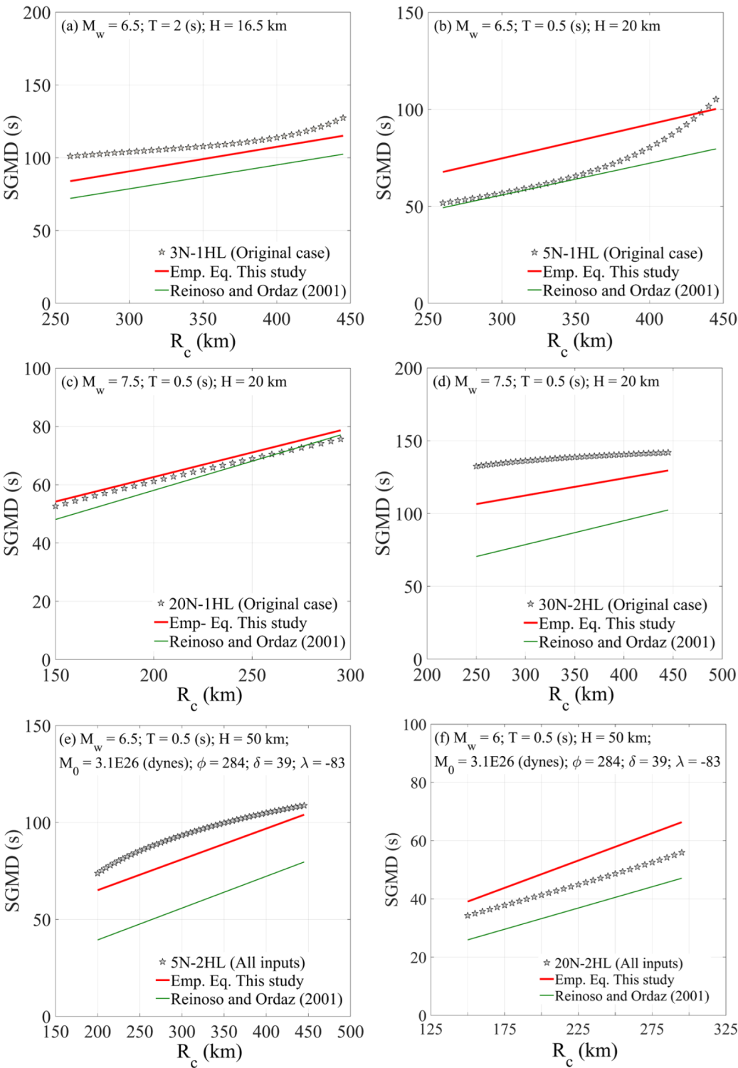
Figure 9 Comparison of SGMD predicted by the trained ANN models and by the empirical models with variation in RC. Interplate events: (a) Mexico City soft soil, (b) Mexico City firm soil, (c) Outside Mexico City firm soil. Inslab events: (d) Mexico City soft soil, (e) Mexico City firm soil, (f) Outside Mexico City firm soil.
To further compare the trained ANN models and the empirical equations, a probabilistic characterization of the error, defined as the difference of the logarithmic of the predicted values of SGMD by using the trained ANN models or the empirical equations for the results presented in Figure 8, and the logarithmic of the observed values is carried out. Figure 10 presents a comparison of the calculated errors in Normal probability paper. It is observed from Figure 10 that the error could be modeled as a normal variate. This was also verified with the Kolmogorov-Smirnov goodness-of-fit test (Benjamin and Cornell, 1970), which indicates that the normality hypothesis could not be rejected at a significance level of at least 1% for both type of seismic events. The mean and standard deviation of the errors presented in Figure 10 are summarized in Table 10. It is observed from Table 10 that the trained ANN models and the empirical equations are only slightly biased and that the statistics of the error for the developed ANN models are similar to those of the empirical equations. Similar results were observed for the ANN models and the empirical equations presented in Figure 9 and for that reason they are not shown.

Table 10 Statistics of the error.
| Type of earthquake | Type of soil | ANN models | Empirical equations | |||
|---|---|---|---|---|---|---|
| Case | Mean | Std. Dev. | Mean | Std. Dev. | ||
| Interplate | SS-MC | All inputs | -3.98E-02 | 0.24 | 2.70E-01 | 0.19 |
| FS-MC | All inputs | 1.07E-02 | 0.31 | 1.01E-01 | 0.38 | |
| FS-M | Original case | -2.03E-02 | 0.21 | 6.39E-03 | 0.3 | |
| Inslab | SS-MC | All inputs | -5.50E-03 | 0.16 | -2.51E-01 | 0.32 |
| FS-MC | Original case | -4.14E-02 | 0.10 | 1.22E-02 | 0.18 | |
| FS-M | All inputs | -1.05E-01 | 0.26 | 1.58E-02 | 0.24 | |
Conclusions
Mexican records from interplate and inslab events were employed to develop Artificial Neural Network models to predict the strong ground motion duration. The principal component method was used to carry out a dimensionality reduction of the input parameters to develop the artificial neural network models. Several ANN architectures were tested. For the training of the ANN models, the input layer considered four different cases (i.e., all inputs, strong relation, moderate relation and original case), while the logarithmic of the SGMD is used to represent the output neuron.
The model tested considered up to 50 hidden neurons with one and two hidden layers. Additionally, new regression coefficients to fit empirical equations to estimate the strong ground motion duration were also obtained. The main observations that can be drawn from the analysis results are:
The analyses results indicated that the best prediction of the SGMD is obtained with ANN models with one hidden layer and 3, 5 and 20 hidden neurons when interplate events are considered; however, when inslab events are considered, the ANN models with two hidden layers and 3, 5, 15, 20 an 30 hidden neurons provide the best predictions.
The best ANN models for interplate and inslab events are associated with the cases referred to as all inputs and original case, which considered 8 and 4 input neurons, respectively. The later indicates that the selection of the inputs neurons is of paramount importance and that the ANN models could improve their prediction ability if the number of input neurons is increased.
The number of neurons per hidden layer of the ANN models that presented the smallest average MSE during the testing process were within 3 to 50.
In general, the predicted values by using the ANN models follow those predicted by the developed empirical equations. This indicates that the ANN models represent a good alternative to the empirical equations in some applications if one does not have to understand the causality to apply the ANN model.
In some cases, the SGMD predicted by using the ANN models presented physically unrealistic trends in its behavior. For this reason, caution is warranted when the model is extrapolated and it is recommended to carry out several verifications of the trained ANN models before using them for further engineering applications, for example the simulation of synthetic records or the evaluation of damage indices.

