


 nueva página del texto (beta)
 Inglés (pdf)
 Artículo en XML
 Referencias del artículo
 Enviar artículo por email
 Citado por SciELO
  Similares en
SciELO
Similares en
SciELO 
 Permalink
Introduction
From the perspective in continuous media mechanics, the advection-dispersion equation (ADE) is the fundamental element to develop a mathematical model that describes the reactive solute transport throughout porous media (Allen et al., 1988; Cao et al., 2020; Fried, 1975; Parker and van Genuchten, 1984; Sorbie et al., 1987; van Genuchten and Parker, 1984). ADE results from total solute mass balance equation, which is obtained by adding the solute mass balance equation on both phases, fluid and solid, and assuming that reaction of solute between both phases is instantaneous, such that local equilibrium is valid, and then it is possible to simplify the expression corresponding to the retardation factor. The implicit physical phenomena are the advection due to drag from the fluid velocity field, which transports the solution, and the hydrodynamic dispersion that accounts for both the mechanical dispersion and the molecular diffusion (Bear, 1988; Bear and Bachmat, 1990). Boundary value problems (BVPs) can be obtained from the ADE, by addition of constraints named boundary conditions specified either on the solute concentration value itself (first-type), on its derivative (second-type) or even on both (third-type); also the boundary conditions are labeled inlet at the injection point and outlet at the withdrawal point, respectively. To describe the complex interrelated phenomena, existing in the reactive solute transport through porous media, non-linear equations are often needed, then an analytical solution is very difficult or even impossible to obtain. However, by establishing some simplifications, it is possible to get analytical solutions, as portrayed in this work.
Studies of solute transport are frequently done by analyzing the solute concentration on effluent samples collected at an observation point. The breakthrough curve is a plot of the effluent concentration versus time (often both dimensionless). Matching the breakthrough curve to a mathematical model available it is possible to obtain the corresponding fitting parameters, such as longitudinal dispersion and retardation factor.
An important part of mathematical models is the appropriate selection of boundary and initial conditions. This topic has been subject of many papers since the initial works in geohydrology, particularly in the case of uniform flow in homogeneous porous media (Gershon and Nir, 1969; Kreft and Zuber, 1978; van Genutchen and Alves, 1982; van Genuchten and Parker, 1984; Parker and van Genuchten, 1986).
Previous studies that evaluated the suitability of prescribed boundary conditions to predict measured solute concentrations in controlled column experiments have addressed the case of saturated flow in artificial and nonreactive media (James and Rubin, 1972; Parker, 1984; Novakowski, 1992b). Outlet effects can be accounted for in the numerical solution to estimate the amount of dispersion that occurs only in the media (James and Rubin, 1972). It has been shown that when local equilibrium between pore regions is not attained, the analytical solution with finite boundaries fails to describe measured concentrations (Parker, 1984). However, for slow pore water velocities, the ADE should provide a good description to experimental data (Schwartz et al., 1999).
The concepts of volume-averaged and flux-averaged concentration were introduced aiming to reproduce real conditions in solute sampling methods (Brigham, 1974; Kreft and Zuber, 1978). Depending on the sampling method it can be necessary to distinguish between volume-averaged and flux-averaged concentrations, which are defined by the mass of solute per elementary volume of the porous media at a given time, and as the mass of solute crossing a unit area per element of time; respectively. In both cases the concentration is defined macroscopically (Novakowsky, 1992a).
BVPs with first-type inlet boundary condition, concentration value prescribed, has been solved for both semi-infinite and finite systems (Danckwerts, 1953; Ogata and Banks, 1961, Lapidus and Amundson, 1952; Cleary and Adrian, 1973). BVPs with third-type inlet boundary condition, flow value prescribed, has been solved for also both semi-infinite and finite systems (Brenner, 1962; Coats and Smith, 1964; Lindstrom et al., 1967). Regarding to outlet boundary condition there are BVPs with first-type, zero concentration value prescribed, only for semi-infinite system (Ogata and Banks, 1961; Coats and Smith, 1964). BVPs with second-type outlet boundary condition, zero gradient concentration prescribed, has been solved for semi-infinite system (Lapidus and Amundson, 1952; Lindstrom et al., 1967). However, the corresponding solution to BVP with second-type outlet boundary condition is the same as the solution to BVP with first-type outlet boundary condition, provided that inlet boundary condition is the same type. That is, BVP-1,1 has the same solution as BVP-1,2; as well as BVP-3,1 has the same solution as BVP-3,2 (see Table 1 for notation). For finite system, the only outlet boundary condition used is second-type (Brenner, 1962; Cleary and Adrian, 1973).
Table 1 Summary of BVPs analyzed.
| Notation | Type of System | Type of Inlet Boundary Condition | Type of Outlet Boundary Condition | Reference to the Analytical Solution |
| BVP-1,1 | Semi-Infinite | First-type Equation (3) | First-type Equation (5) | Ogata and Banks, 1961. |
| BVP-1,2 | Semi-Infinite | First-type Equation (3) | Second-type Equation (4) | Lapidus and Amundson, 1952. |
| BVP-3,1 | Semi-Infinite | Third-type Equation (2) | First-type Equation (5) | Coats and Smith, 1964. |
| BVP-3,2 | Semi-Infinite | Third-type Equation (2) | Second-type Equation (4) | Lindstrom et al., 1967. |
| FBVP-1,2 | Finite | First-type Equation (3) | Second-type Equation (8) | Cleary and Adrian, 1973. |
| FBVP-3,2 | Finite | Third-type Equation (2) | Second-type Equation (8) | Brenner, 1962. |
Defining appropriate boundary conditions between porous and non-porous media is not a simple subject (Parker and van Genutchen, 1986). Several efforts have been performed to determine the real type of boundary conditions that apply in solute transport experiments through porous columns (van Genutchen and Parker, 1984; Novakowski, 1992a,b; Schwartz et al., 1999). Results indicate that to certain extent third-type inlet boundary condition can better describe laboratory data than first-type inlet boundary condition can. Some apparently innocuous first-type boundary condition result in solutions that are mathematically correct but physically incorrect, since they yield improper mass balance and pulse behavior (Coronado et al., 2004). This might be the reason why models based on some first-type inlet boundary conditions have failed in matching experimental data.
This paper remarks some warnings about using solutions of ADE to describe reactive solute transport through porous media. In the next section, the ADE is introduced and a discussion about various solutions available in both semi-infinite and finite systems is given. The next section shows some results based on breakthrough curves for every analytical solution available. A parametric analysis with the Peclet number is done to observe the range of values where a good approximation between solutions is obtained. Conclusions and suggestions are provided in the final section.
Theory
The governing equation to describe reactive solute transport with linear and reversible equilibrium adsorption through homogeneous porous media, during saturated flow, is the called ADE:
where
Solutions
In order to obtain analytical solutions of ADE , some simplifying assumptions are needed to decrease the complexity of the problem. Neglecting molecular diffusion, the solute transport is basically hydrodynamic. The injection of solute into the inlet boundary is such that solute velocities are proportional to velocities of the particular flow paths causing concentration to be weighted by the combined flow rates of all flow paths. On these conditions it is agreed that the correct inlet boundary condition for flux injections of solution with a prescribed concentration
which is a third-type specified flux boundary condition that is required by mass conservation across the inlet boundary condition.
However a first-type specified concentration boundary condition has also been used frequently:
This condition implies a usually not possible in practice situation, the concentration itself needs to be specified at the porous media surface. Moreover the solutions obtained with this condition not satisfied mass conservation.
For a semi-infinite system, the outlet boundary condition specify the behavior of the concentration as infinity is closer. It is plausible that change in concentration with respect to distance are negligible as distance goes to infinity, thus the outlet boundary condition is ( van Genutchen and Parker, 1984; Schwartz et al., 1999):
Furthermore first-type specified zero concentration outlet boundary condition can be as (Ogata and Banks, 1961):
To use a first-type specified zero concentration outlet boundary condition might be easier than a second-type zero gradient outlet boundary condition, both analytically and numerically.
For a finite system, one requirement that always must be satisfied is continuity of the solute velocity across the outlet boundary condition (van Genutchen and Parker, 1984):
where
Assuming that the solute concentration should be continuous across the outlet boundary:
Therefore, the outlet boundary condition (6) results in:
which is a second-type zero-gradient outlet boundary condition, almost always used (Brenner, 1962; Cleary and Adrian; 1973).
To complete the different BVPs to be analyzed here, the initial condition that describe a porous media system free of solute is used:
Table 1 summarizes the various BVPs, which could be defined with the above boundary and initial conditions.
For a semi-infinite system, the first BVP listed on Table 1, called BVP-1,1, have the inlet boundary condition (3), the outlet boundary condition (5) and the initial condition (9); which analytical solution for ADE is adapted from Ogata and Banks (1961):
The second BVP on Table 1, called BVP-1,2, has the same inlet boundary condition (3) and initial condition (9) as the first one, but the outlet boundary condition is now . Its analytical solution, adapted from Lapidus and Amundson (1952), is the same as the solution for ADE , adapted from Ogata and Banks (1961). For this reason, only one will be presented.
The BVP-3,1 is defined using the inlet boundary condition , the outlet boundary condition (5) and the initial condition condition (9). Its analytical solution is taken from Coats and Smith (1964):
The BVP-3,2 is like the previous one, but using the outlet boundary condition (4). The analytical solution is given by Lindstrom et al. (1967) and is the same as the analytical solution adapted from Coats and Smith (1964). For this reason, only one will be presented.
Expressions for the effluent concentration
For a finite system, similar problems can be defined. Thus the problem with the inlet boundary condition (2), the outlet boundary condition (8), and the initial condition (9); is the FBVP-3,2 which have the analytical solution adapted from Brenner (1962):
where
The FBVP-1,2 is like the previous one, but using the inlet boundary condition (3); and have the analytical solution adapted from Cleary and Adrian (1973):
where
Expressions for the effluent concentration
In order to compare the solutions for the semi-infinite system with the solutions for the finite system, the position of the outlet boundary condition is denoted by
Results and discussion
Dimensionless variables are used to solute concentration,
Figure 1 shows the breakthrough curves corresponding to the analytical solutions for the different initial and boundary value problems described above. The Peclet number was chosen equal to 1 to increase the differences among the solutions because, as can be seen in Figure 2, for a Peclet number equal to 20, some breakthrough curves become practically indistinguishable. It can be observed that analytical solutions approach each other as Peclet number grows, such that differences between them are practically negligible for a Peclet number greater than twenty. Note that only four curves are shown because two solutions are identical to another two, specifically BVP-1,1 has the same solution as BVP-1,2; as well as BVP-3,1 has the same solution as BVP-3,2.
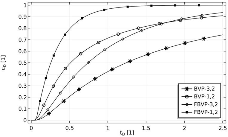
Figure 1 Breakthrough curves for semi-infinite systems (BVP) and finite systems (FBVP). The Peclet number equals 1.

Figure 2 Breakthrough curves for semi-infinite systems (BVP) and finite systems (FBVP). The Peclet number equals 20.
The Peclet number is used to do a parametric analysis for each problem in Table 1. Figure 3 shows the breakthrough curves for the FBVP-3,2 depending on the Peclet number. For a finite system, the position of the outlet boundary condition is the same as the measurement position,

Figure 4 shows the breakthrough curves for the BVP-3,2 depending on the Peclet number. In this case, the position of the outlet boundary condition goes to infinity.
In Figure 5, observe how, as the position of the outlet boundary condition goes from the measurement position to infinity, the breakthrough curves go from the analytical solution for the finite system to the analytical solution for the semi-infinite system.
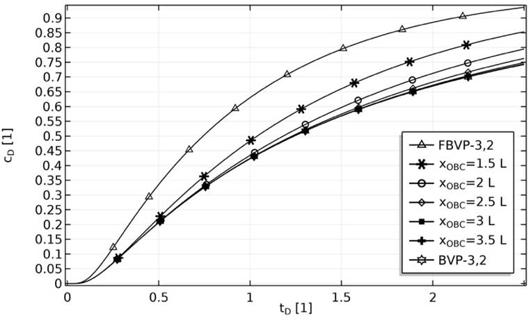
Figure 5 Breakthrough curves for the FBVP-3,2 and the BVP-3,2; and transition between them as the position of the outlet boundary condition goes from the measurement position to infinity. The Peclet number equals 1.
Figure 6 shows the breakthrough curves for the FBVP-1,2 depending on the Peclet number. For a finite system, the position of the outlet boundary condition is the same as the measurement position,

Figure 7 shows the breakthrough curves for the same problem as above, but for a semi-infinite system, it is a BVP-1,2. In this case, the position of the outlet boundary condition goes to infinity,

In Figure 8, observe how, as the position of the outlet boundary condition goes from the measurement position to infinity, the breakthrough curves go from the analytical solution for the finite system to the analytical solution for the semi-infinite system.
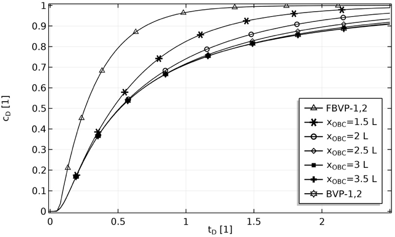
Figure 8 Breakthrough curves for the FBVP-1,2 and for the BVP-1,2; and transition between them as the position of the outlet boundary condition goes from the measurement position to infinity. The Peclet number equals 1.
It is very important to estimate the Peclet number, for each experimental or field test, to have confidence about using analytical solutions of ADE to describe solute transport through porous media. Be aware of which solution may be more appropriate to describe data obtained from a real breakthrough curve because, as is shown here, there may be significant differences between them; and then get misleading parameters from the matching procedure.
Conclusions
Analytical solutions for different BVPs defined by de ADE with various combinations of inlet and outlet boundary conditions, and the initial condition corresponding to a free of solute, both finite and semi-infinite systems, had been analyzed systematically. All the available analytical solutions are plotted together to observe their behavior for a Peclet number equal to one (Fig. 1) and for a Peclet number equal to twenty (Fig. 2). From this comparison, it is concluded that much thoughtfulness must be taken to choose the most suitable analytical solution to describe the transport of reactive solute through porous media when the system to be studied has a Peclet number smaller than five. However, when the system under research has a Peclet number greater than twenty, the differences between all solutions available are practically negligible and therefore any of them could be useful. It is important to remark that, even though, the analytical solution for the BVP-1,1 is the same as the analytical solution for the BVP-1,2, as well as, the analytical solution for the BVP-3,1 is the same as the analytical solution for the BVP-3,2 it is generally easier to compute, to use, and to implement, the former than the latter. That is because an outlet boundary condition type-1 prescribes the variable value directly instead of prescribing its derivative as an outlet boundary condition type-2 does. Even more, when a numerically solution is to be implemented, some advantage could be obtained if an outlet boundary condition type-1 is used, instead of a type-2.
It is possible to observe the behavior of the solutions going from the solution for the finite system to that for the semi-infinite system, moving the location of the outlet boundary condition from the observation or measurement location, where
Based on the parametric analysis done, it is advisable that system studied has a Peclet number at least of five, confirming suggestions by other authors (e.g.van Genutchen and Parker, 1984; Parlange et al., 1985; Coronado and Ramirez-Sabag, 2005), in order to confidently use the solutions mentioned above. Also could be observed in Fig. 2 that for Peclet number greater than twenty, there are not significant difference between the revised solutions, therefore there are not preference to use anyone of them.

