


 nueva página del texto (beta)
 Inglés (pdf)
 Artículo en XML
 Referencias del artículo
 Enviar artículo por email
 Citado por SciELO
  Similares en
SciELO
Similares en
SciELO 
 Permalink
Introduction
The Gulf of California (GoC) is obliquely rifted that connects the East Pacific rise spreading ridge in the south with the San Andreas Fault in California. The trans-tension between the North American and Pacific plates resulted in the generation of the large earthquakes in the GoC along with the transform faults and the spreading ridges (Castro et al., 2011b; Castro et al., 2017b). The earthquakes in this region follow a fairly linear trend along the southeastward direction from southern California to the southern end of the Gulf of California, Mexico. The transform faults are associated with right lateral strike slip faulting while normal faulting is observed near the spreading centres. The northern GoC comprises the complex transform fault geometry and is the major reason for large (Ms > 6) earthquakes in this region (Goff et al., 1987, Castro et al., 2017b). The observed mechanism of faulting in this region is oblique -normal faulting in nature (Persaud et al., 2003, Castro et al., 2017b). On the other hand, the southern GoC comprise the ridge transform fault system along with the hot zones under the weak crust is the dominant mode of rupturing to generate large (Mw: 7.0 (January 7, 1901)) earthquakes (Pacheco and Sykes, 1992). These factors along with the oblique plate motion also resulted in the rapid rupturing of southern region (Umhoefer 2012).
Seismic waves generated from an earthquake experienced the attenuation of wave amplitude at distant locations from the source. The attenuation rate of seismic wave amplitude is very sensitive to the presence of fluids in the rocks, temperature conditions, the composition of rocks and other factors, while propagating through the earth interior. Local geology or the site condition at a location also plays a key role during an earthquake by amplifying or attenuating the seismic waves at different sites. The seismic attenuation is described in terms of inverse of a dimensionless parameter known as the Quality factor (Knopoff 1964). In 1984, Hasida and Shimazaki introduced a technique to estimate the 3D Q-structure using the intensity data for Tohoku region, Japan. Later Satake and Hasida (1989) and Nakamura and Uetake (2002) has used this method to distinguish and understand the behaviour of low and high attenuation regions for north Island, New Zealand and Pacific sea plate, Japan. Besana et al., (1997) has studied the regional effects of subsurface structures like arcs, slabs and continental material using the 3D Q-structure for Philippine region. Later, Nakamura and Uetake (2002) and Joshi et al., (2010) has modified the technique and use the acceleration data to obtain the attenuation structure for Tohoku, Japan and Uttarakhand, India regions. Attenuation studies around the world based on Q -1 values have been used to characterize the tectonic regions e.g. stable, volcanic, and seismically active (Joshi et al., 2010; Castro et al., 2008; Kumar et al., 2015). The less attenuating media in a region is characterized by the high Q value and the vice versa.
Various attempts have been made to understand the attenuation behaviour of seismic waves in GoC and the surrounding region. For the southern region, Ortega and González (2007) has followed the general least square regression of strong motion data to determine the S or Lg wave attenuation for the La Paz-Los Cabo region, Baja California, Mexico. The obtained results were further validated, using the coda normalization method and reported a lower attenuation for the La Paz-Los Cabo inland region. Later, Ortega and Quintanar (2011) used the offshore earthquake data and compared the propagation characteristics of S waves reported by Ortega and González (2007) with the P wave propagation characteristics following the same method. Vidales-Basurto et al., (2014) has conducted the attenuation study in the south central GoC region to understand the tectonic structure of gulf region. The results obtained based on the different source receiver distance depicts the higher body wave attenuation along the oceanic spreading centres. Also, high attenuation is observed towards the southern gulf region compared to the central gulf region. Later, Rodríguez-Lozoya et al., (2017) estimated the coda attenuation for central gulf region and observed a similar higher attenuation for the southern sub region. Also, Castro et al., (2017b) determined the body wave attenuation and source functions for the gulf region using the foreshocks, aftershocks and the main shock (Mw= 6.6) of event occurred on October 19, 2013, along the Farallon fault region. For central gulf region, Quintanar et al., (2019) have analysed the foreshocks, main shock (Mw=6.6) and aftershocks of January 4, 2006 San Pedro Martir earthquakes. They obtained the source parameters, fault geometry and fault slip distribution for the earthquake and later used them to study the attenuation behaviour of gulf region. More, recently Castro et al., (2019) studied the one-dimensional variability of Qs in the southern region of GoC at selected frequencies. They reported an increase of Qs with increase of frequency but small variation of Qs has been observed with depth (5-40 km) at individual frequencies.
The present article uses the approach given by Joshi et al., (2010) to obtain three- dimensional attenuation structure in a broad frequency range. We use data from 25 earthquakes recorded both onshore and offshore by Ocean Bottom Seismographs (OBS) deployed in the study area of south-central Gulf of California (GoC) region. This tectonically complex region comprises a system of short spreading centres and transform faults and is considered as a high seismicity zone (Sumy et al., 2013). The attenuation structure must have a strong correlation with the tectonic environment and the seismic wave velocity (Lizarralde et al., 2007; Luccio et al., 2014) and for this reason, is important to evaluate the attenuation characteristics of GoC.
Tectonic structure of study area
The Gulf of California (GoC) is relatively young, oblique rift system that formed with the cessation of the Farallon plate subduction under the North American plate about 12 million year ago (Lonsdale, 1989). The evolution of the GoC extensional province occurred in two stages; stage-I: extension and separation of the continents that resulting in the formation of marine basins; stage-II: is being continued till today is the expansion of seafloor and structure of transform faults (Stocks and Hodges 1989; Bennett et al., 2007; Vidales-Basurto et al., 2014). The GoC is comprised a group of stepping faults, seafloor spreading, ridges and the right lateral strike-slip transform faults which collectively form a continental rift system. Consequently, it facilitates the Pacific Plate to move apart from the North American plate. However, an anomalous left lateral strike slip faulting has been observed for September 1, 2007 main shock (Mw= 6.1) and its subsequent aftershocks activities in the southern gulf region (Ortega & Quintanar, 2010). The unusual characteristics of main shock and the high rate of aftershock (more than 800 during a period from September to December 2007) activities for a transform fault is believed to be a combination of narrow bathymetry, growing seafloor and stress interaction along the continental oceanic transition (COT) boundary. The major tectonic faults and the corresponding oceanic basins in GoC is shown in Fig 1. The crust underneath the ocean basins in GoC differs in terms of thickness, rifting style, sea floor spreading, and magmatism.
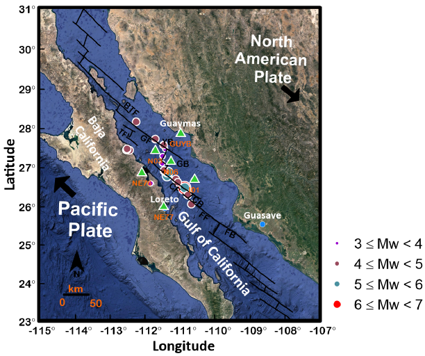
Figure 1 Map showing the location of recording stations (green triangles) and epicentres (circles) of the earthquakes selected. The purple, brown, sea green and the red circle are different magnitude bins and has been scaled as per the magnitude of earthquakes. The location of faults is taken from Aragon-Arreola et al., (2005) and Dorsey et al., (2013). DB= Delfin Basin, BTF= Canal de Ballenas Transform Fault, YB= Yaqui Basin, GF= Guaymas fault, GB= Guaymas Basin, CF= Carmen Fault, CB= Carmen Basin, FF= Farallon Fault, FB= Farallon basin, TF= Tortuga Fault. The black arrows represent the plate motion.
The south central GoC has a distinct rifting style compare to the surrounding region. Lizarralde et al., (2007) has observed that evolution of rifting in this region is primarily controlled by the magmatic depletion of mantle. The anomalous Guaymas basin in the central region is considered as magmatic since the beginning of breakup (~ 6 m.a.) and possess the largest new igneous crust spread over ~280 km. The intrusive magmatism in the overlain sediments has resulted in the formation of sills over a large distance from the spreading centre (Aragón-Arreola et al., 2005). On the other hand, the Farallon and Pescadero segment in the south of Guyamas basin have narrow ocean basins with nascent or no sea floor spreading (Lizarralde et al., 2007).
Data Used
The highly active south-central GoC was monitored by regional seismic network of NARS- Baja (Network of Autonomously Recording Seismographs) and the Broadband Network (RESBAN) operated by the CICESE (Avila-Barrientos and Castro, 2016). The present study also used some of the events recorded offshore by eight Ocean bottom Seismographs (OBS’s) deployed under the Sea of Cortez Ocean Bottom Array (SCOOBA) experiment in the Guaymas and Alarcon basins (Sumy et al., 2013). This offshore network was operative only from October 2005 to October 2006. For the present study, 25 earthquakes recorded on both onshore and offshore stations deployed in the GoC were used. The offshore OBS’s are equipped with four components (two horizontal, one vertical and one pressure component) to record the ground motion at the recording rate of 32.25 samples/s (Sumy et al., 2013). The onshore broadband system, operated by CICESE, is equipped with three-component sensors, recording at 20 samples/s (Castro et al., 2017b, 2018). The recording stations and the epicentral location of the earthquakes used in this study are shown in Fig. 1. The calculated hypocentral parameters of the selected earthquakes and the stations used are listed in Table 1.
Table 1 Parameters of earthquake used in the present work.
| S. No. | Year | Month | Day | Hour | Minute | Second | Latitudeo | Longitudeo | Depth (km) | Magnitude (Mw) | Recording Stations |
|---|---|---|---|---|---|---|---|---|---|---|---|
| 1 | 2002 | 12 | 6 | 6 | 24 | 12.256 | 26.3152 | -110.7364 | 8.6 | 4.0 | GUYB, NE76, NE77 |
| 2 | 2002 | 12 | 7 | 1 | 33 | 45.285 | 26.0794 | -110.633 | 9.8 | 4.1 | GUYB, NE76, NE77 |
| 3 | 2002 | 12 | 8 | 17 | 45 | 17.391 | 26.3141 | -110.7159 | 16.2 | 3.5 | GUYB, NE76, NE77 |
| 4 | 2003 | 1 | 19 | 16 | 46 | 30.147 | 26.9204 | -111.3973 | 2.0 | 4.0 | GUYB, NE76, NE77 |
| 5 | 2003 | 3 | 12 | 23 | 41 | 30.561 | 26.4994 | -110.8355 | 2.0 | 6.3 | GUYB, NE76, NE77 |
| 6 | 2003 | 3 | 13 | 4 | 23 | 7.463 | 26.4337 | -110.7387 | 8.3 | 4.0 | GUYB, NE76, NE77 |
| 7 | 2003 | 3 | 13 | 14 | 38 | 20.61 | 26.6403 | -111.0145 | 15.6 | 4.1 | GUYB, NE76, NE77 |
| 8 | 2003 | 3 | 22 | 17 | 55 | 41.519 | 26.5048 | -110.8193 | 5.3 | 4.8 | GUYB, NE76, NE77 |
| 9 | 2004 | 2 | 18 | 19 | 30 | 39.033 | 26.6345 | -111.0169 | 7.2 | 3.9 | NE76, NE77 |
| 10 | 2004 | 8 | 7 | 10 | 41 | 24.442 | 26.6103 | -111.7947 | 6.2 | 3.2 | GUYB, NE76, NE77 |
| 11 | 2006 | 4 | 20 | 3 | 40 | 41.28 | 28.194 | -112.21 | 3.0 | 4.0 | GUYB, I01, N03, NE76, NE77 |
| 12 | 2006 | 4 | 23 | 7 | 50 | 40.05 | 27.498 | -111.38 | 4.0 | 3.6 | GUYB, I01, N03, N06, NE76, NE77 |
| 13 | 2006 | 5 | 11 | 5 | 58 | 18.04 | 27.311 | -111.45 | 1.0 | 3.9 | I01, N03, N06, NE76, NE77 |
| 14 | 2006 | 5 | 28 | 14 | 0 | 56.78 | 26.948 | -111.41 | 12.0 | 4.8 | GUYB, NE76, NE77 |
| 15 | 2006 | 5 | 28 | 14 | 18 | 2.23 | 26.904 | -111.3 | 4.0 | 5.3 | GUYB, NE76, NE77 |
| 16 | 2006 | 6 | 11 | 4 | 11 | 36.33 | 26.726 | -111.08 | 5.0 | 4.2 | I01, N03, N06, NE77 |
| 17 | 2006 | 6 | 16 | 8 | 46 | 44.74 | 27.595 | -111.42 | 2.0 | 4.5 | I01, N03, N06, NE76, NE77 |
| 18 | 2006 | 7 | 30 | 1 | 20 | 56.96 | 26.809 | -111.326 | 19.4 | 5.9 | GUYB, NE76, NE77 |
| 19 | 2006 | 8 | 7 | 2 | 50 | 53.05 | 27.503 | -112.47 | 6.0 | 4.3 | I01, N03, N06, NE76, NE77 |
| 20 | 2006 | 8 | 8 | 4 | 29 | 32.29 | 27.472 | -112.49 | 5.0 | 4.3 | I01, N03, N06, NE76, NE77 |
| 21 | 2006 | 8 | 8 | 21 | 36 | 35.8 | 27.461 | -112.39 | 10.0 | 4.1 | I01, N03, N06, NE76, NE77 |
| 22 | 2006 | 8 | 9 | 23 | 32 | 19.38 | 27.485 | -112.47 | 5.0 | 4.3 | I01, N03, N06, NE76, NE77 |
| 23 | 2006 | 8 | 11 | 17 | 55 | 11.5 | 26.881 | -111.34 | 5.0 | 4.2 | I01, N03, N06, NE76, NE77 |
| 24 | 2006 | 9 | 12 | 18 | 56 | 28.36 | 27.753 | -111.66 | 2.0 | 4.0 | I01, N03, N06, NE76, NE77 |
| 25 | 2006 | 9 | 25 | 13 | 4 | 5.65 | 27.122 | -111.46 | 5.0 | 3.9 | I01, N03, N06, NE76, NE77 |
Fourier amplitude spectra of S-wave windows from 98 records have been used as an input in the inversion. The spectral input files consist of 18 discrete values of S-wave spectral amplitudes that range from 0.16 Hz to 7.94 Hz. Fig. 2 shows a sample of the amplitude spectra of a few stations along with the epicentral distance (ED). The earthquakes selected were relocated by Castro et al., (2011) using records from the regional stations of the NARS-Baja (Trampert et al., 2013) and RESBAN (Castro et al., 2018b) arrays. Some of the events were located by Sumy et al., (2013) using OBS’s. Fig. 3 represents the magnitude hypocentral distance plot for selected events. The records were corrected for instrument response and they were baseline corrected. The S-wave windows length used to calculate the fourier amplitudes amplitudes varies between 2 s for local hypecentral distance to 75 s for regional distance. The time window starts a few seconds before the first S-wave arrival and ends before the surface waves arrive. The spectral records were smoothed choosing 20 equidistant frequencies, between 0.16 and 7.94 Hz, on a logarithmic scale and averaging the amplitudes using a variable frequency band of ± 25% over the central frequencies chosen (Castro et al., 2017a).
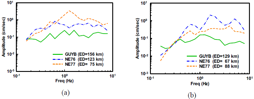
Figure 2 Amplitude spectra of S-phase recorded at stations GUYB, NE76 and NE77 from the following earthquakes: (a) 12/03/2003 (Mw=6.3) (b) 30/07/2006 (Mw=5.9)
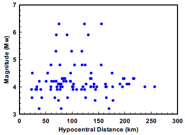
Figure 3 Spatial distribution of magnitude versus hypocentral distance of analyzed earthquakes. The selected earthquakes have Mw ranging from 3.2 to 6.3 with hypocentral distance from 20 km to 260 km.
The site response functions determined by Vidales-Basurto et al., (2014) and Avila-Barrientos and Castro (2016) for both the NARS-Baja and the RESBAN broadband stations were used to correct the spectral amplitudes for site effects.
A rectangular block of dimension 230 km to 288 km was selected on the basis of coverage area of seismic network and availability of events within it. This block is divided into six sub-blocks with individual sub-block having a rectangular area 38 km x 48 km. These blocks are further extended by three blocks of thickness upto a depth of 12 km; thereby dividing entire area into individual three dimensional blocks of size 38 km x 48 km x 4 km. The location of the rectangular block is shown in Fig. 4 along with the structural features of the study region. Inset zoom in the Fig. 4 represents the straight-line ray path projection in sub blocks between the events and the recording stations. The spectral amplitudes shown in Fig. 2 are from earthquake located between the first and third row of considered rectangular block.
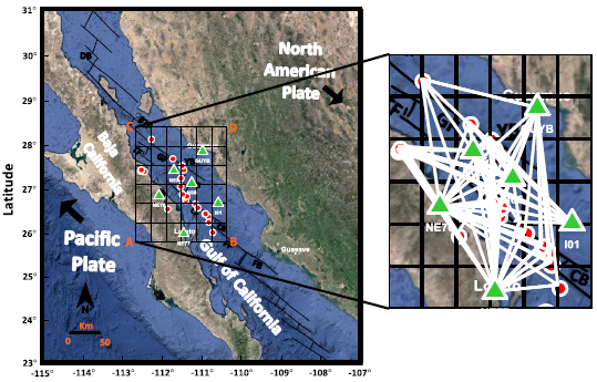
Figure 4 Map with location of the study area and the rectangular grid (ABCD) of the volume sampled, along with the tectonic features in the rectangular grid (ABCD). Red circles with white boundary indicate the epicentres of selected earthquakes. Inset zoom shows the projection of ray paths between the selected events and the recording stations in the studied area.
Methodology
The inversion procedure used is based on the method proposed by Aki and Lee (1976). A cartesian co-ordinate system has been used to represent the distribution of the shear wave attenuation coefficient of the study region. The region was divided into 108 rectangular blocks with each block having a different Q s (f) value. The corners of these rectangular blocks on the surface of the Earth are assumed as the observation points. For an earth model having several blocks with different shear wave attenuation coefficient values, Qs(f) for a given frequency f, the spectral acceleration A(f) can be given by the following relation (Hashida and Shimazaki 1984):
Where S(f) denotes the source acceleration at frequency f, G represents the geometrical spreading function and R the hypocentral distance, ga is site amplification term and Tijr represents the travel time of the ray in rth block having attenuation coefficient Cpqr. The parameter Qr(f) represents the frequency dependent quality factor in the rth rectangular block. The subscript i, j represents the ith station and the jth event, respectively. To solve equation (1), an initial three dimensional Qpqr,o(f) model of earth is assumed. The subscripts p, q is used to define the blocks along the two-horizontal directions of the rectangular area as shown in Fig. 5. The subscript r identifies the rectangular blocks in the downward direction. The initial input model is based on the velocity and Qs models (Rebollar et al., 2001 and Paulseen and de Vos (2017)) available for the studied region. The initial guess of source strength Scal(f) for inversion has been calculated using initially assumed Q model and recorded spectral acceleration in the following relation:
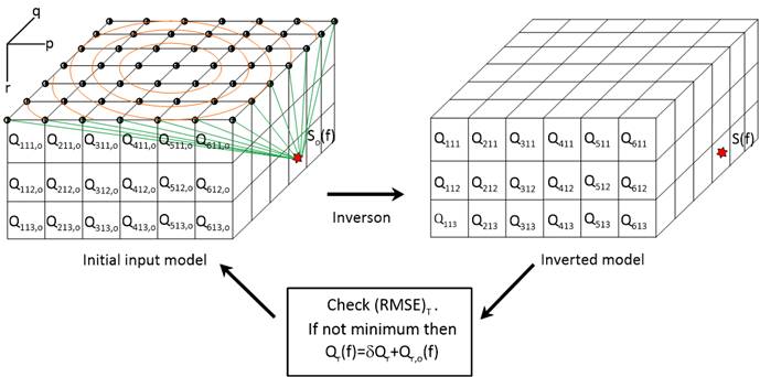
Figure 5 Schematic representation of inversion of initial Qpqr,o model used to obtain the final Qpqr model for different rectangular blocks. The orange circles represent the spectral acceleration contours at frequency f and is used to obtain the calculated spectral acceleration Aijcal(f). Red star and half black circles symbolize the theoretical position of earthquake and the observation points, respectively. Green lines depict the theoretical straight line ray path from source to the observation points through the different Qpqr model blocks in time Tijpqr.
Where
If the observed spectral acceleration at any point is defined as
Natural logarithms on both the sides of above equation gives the following equation:
Where
“Resij (f)” represents the residual acceleration and is used as a known variable for the inversion process. The term e stands for error in calculation.
The parameters δCpqr and Tijr on the right-hand side of equation (4) can be calculated from the
initial velocity model using ray theory. For a particular earthquake, the total
number of equations corresponds to the number of observation points. In equation (4),
The process of obtaining spectral acceleration at each point in the grid is obtained directly from an inbuilt subroutine that calculates contour values at different positions using the spectral data of S phase from each record analysed. Fourier amplitude spectra of 98 records has been used to obtain 18 three dimensional structures in the discrete frequency range from 0.16 Hz to 7.94 Hz.
Tests for Input parameter
The results of the inversion depend on the quality of input data (e.g. Joshi 2007). In the present work, the input data consists of the initial velocity model, the initial shear wave attenuation model, hypocenters distances and distribution of the selected events and the S- wave window chosen to calculate the spectral acceleration values. To test the sensitivity of these parameters, various input parameter tests were performed, like the effect of the velocity model and the resolution of the final attenuation model on the input parameters.
Bakus and Gilbert (1968) have used the resolution matrix to check the suitability of model matrix, which can be defined for the damped least-square inversion using the following relation:
Where R represents the resolution matrix and when R equals to the unit matrix, the obtained solution is unique. As the resolution matrix deviates from the unit matrix, the resolution becomes poorer. Several attempts had been made to check the resolution matrix for simple cases, and the obtained results are close to identity matrix for damped least-square inversion method. This simple case is also used for testing the reliability of the developed algorithm for inversion. For the actual case of acceleration data, the final model is selected based on the minimization of root mean square errors (RMSE). The RMSEA between the observed and calculated spectral acceleration at a particular frequency is given by the following equation:
Where Aical and Aiobs denote the calculated and the observed spectral acceleration values at N number of observation points. The RMSE between the observed and calculated data and model matrix can also be computed using the equation (6). A reliable solution is obtained when all the errors are minimized simultaneously. The final model is selected based on the minimization of the following equation:
Where Nor(RMSE)dat and Nor(RMSE)mod represents the normalized RMSE due to data and model matrix. However, it is hard to minimize Nor(RMSE)dat, (RMSE)A and (RMSE)mod simultaneously for the same iteration, that is (RMSE)T always differs from the ideal value equal of one. Moreover, the choice of the initial model and the number of input events also plays a vital role to obtain the final solution.
Test for Velocity model
Results of inversion depend upon the appropriate velocity models used for the parameterization of earth’s structure as the properties mainly change with depth due to compaction, sedimentation and thermal changes. A numerical experiment was performed to check the distribution of shear wave velocity (Vs) model and quality factor (Qs) value for one layer, two layers and three layers model. The initial velocity model with different Qs values is shown in Table 2. The input models are based on the velocity and Qs models used by Rebollar et al., (2001) and Paulseen and de Vos (2017) for the Gulf and Baja California region. The final model selection is based on the minimization of (RMSE) T. In the present work, error reduces from 252 x 10-4 to 134 x 10-4 when model changes from homogeneous to three layer model. Table 3 shows error estimates for homogeneous and layered earth models. Fig. 6 shows the dependency of the final attenuation structure on the initial velocity model and their corresponding error estimates. The three models predict a local high Qs zone but is located more accurately for two and the three-layer models. The 3-layer model provides more details of the Qs structure and fits the data better.
Table 2 Initial homogeneous layer, two layer and three layer earth models.
| Depth (km) | Velocity (km/s) | Qs | Velocity (km/s) | Qs | Velocity (km/s) | Qs |
|---|---|---|---|---|---|---|
| 0-4 | 2.83 | 40 | 2.83 | 20 | 3.27 | 50 |
| 4-8 | 3.18 | 50 | 3.49 | 65 | 3.27 | 50 |
| 8-12 | 3.80 | 90 | 3.49 | 65 | 3.27 | 50 |
Table 3 Estimate of (RMSE)T and its iteration for homogeneous layer, two layer and three layer earth model.
| Initial earth model | Minimum (RMSE)T (10-4) | Number of iterations corresponding to final model |
|---|---|---|
| Homogeneous layer | 252 | 2 |
| Two layer | 179 | 3 |
| Three layer | 134 | 3 |
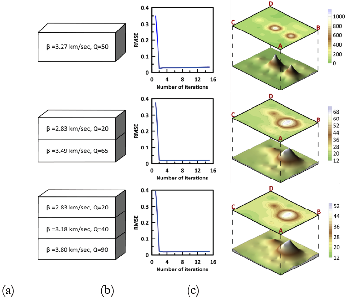
Figure. 6 Dependency of final attenuation structure on the initial velocity models with different Q values. (a) represents the initial layer model, (b) the error corresponding to input layer model and (c) the surface layer (0-4 km) attenuation structure contours along with the 3D projection of contour values at 1 Hz frequency.
Test for input datasets
In this experiment, the behaviour of the number of input earthquake data on final attenuation structure has been studied by removing some input earthquakes sequentially. The final attenuation model obtained using the data set of ten, fifteen and twenty-five earthquakes are shown in Fig. 7. This figure shows horizontal projections of the Q estimates obtained at different depths (0-4 km, 4-8 km and 8-12 km). Since the three data sets used for this test sample different crustal volumes, the resulting Q contours are significantly different. It is clear that the greater the number of sources used the better is the fit and the convergence. Table 4 shows error estimate and the number of iterations corresponding to the final solution for ten, fifteen and twenty-five earthquakes data sets, respectively. It is observed from the inversion that the (RMSE)T decreases with increase in input earthquake data and attenuation structure become much visible compared to that obtained using fewer earthquakes.
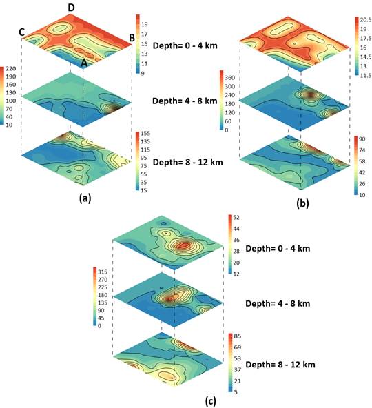
Figure 7 Dependency of the final attenuation model on the number of input earthquake data. Final models obtained for input data set of (a) Ten (b) Fifteen and (c) Twenty-Five earthquakes.
Results and discussion
The geologically young and tectonically complex region of the GoC provides an opportunity to understand the attenuation characteristics of the crust in this region. We have determined a three-dimensional (3-D) attenuation structures for the south - central GoC region. The area of interest has been divided into the 108, 3-D rectangular blocks of dimensions 38 km x 48 km x 4 km. The selection of dimensions of the rectangular blocks is based on the location of recording stations and earthquake epicentres. All stations and hypocenters of earthquakes lie within these rectangular blocks.
In the present article, the three - dimensional attenuation structure has been determined from a total of 1944 estimates of the shear- wave quality factor at 18 discrete frequencies. The resolution matrix of the inversion has significant importance in understanding how much information has been recovered in individual blocks. Fig. 8 is a 2-D view of the resolution matrix for the individual blocks. Blocks with resolution value > 0.7 have been considered as well resolved, and it has been observed that almost all the blocks in the region sampled are in general well resolved. Fig. 9 displays the source-station ray paths and illustrates the coverage of the volume sampled, which is good at depths above 10 km.
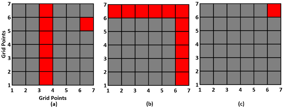
Figure 8 Block diagram representing the resolution matrix values obtained in individual blocks from the inversion at (a) 0 - 4 km depth, (b) 4 - 8 km depth and (c) 8 -12 km depth, respectively. Grey color blocks are well resolved (resolution value > 0.7) while the red blocks are poorly resolved (resolution value < 0.7).
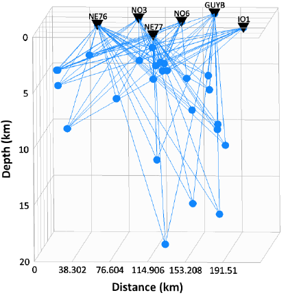
Figure 9 Ray-path diagram illustrating the coverage of different blocks between the events and their respective recording stations. The events are represented by the blue dots and the station shown by the inverted black triangles.
The inversion algorithm gives three-dimensional attenuation structure at 18 different frequencies at which spectral input data has been used. The three-dimensional attenuation structure at 0.5 Hz, 1.0 Hz and 2.0 Hz, respectively, are shown in Fig. 10, 11 and 12. The blocks with low-resolution values have been covered with white blocks.
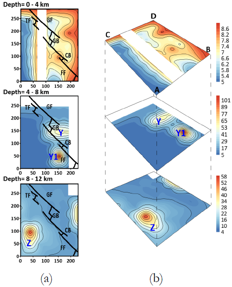
Figure 10 Quality factor contours obtained from the inversion at 0.5 Hz frequency for (i) 0-4 km (ii) 4-8 km (iii) 8-12 km depths. The solid line in (a) represents the tectonic features present in the study region. Labels Y, Y1 and Z represent the high Q patches observed at various depths. Blocks of lower resolution are covered by the white rectangular blocks.
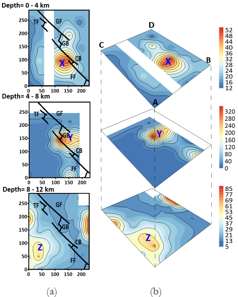
Figure 11 Quality factor contours as in Fig. 9 but at 1.0 Hz for (i) 0-4 km (ii) 4-8 km (iii) 8-12 km depths. The solid black line in Fig. (a) represents the tectonic features present in the study region. Labels X, Y and Z points out high Q patches observed at various depths. Blocks of lower resolution are covered by the white rectangular blocks.
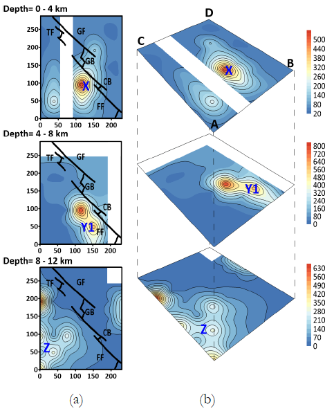
Figure 12 Quality factor contours at 2.0 Hz for (i) 0-4 km (ii) 4-8 km (iii) 8-12 km depths. The solid line in (a) represents the tectonic features present in the study region. Labels X, Y1 and Z points out the high Q patches observed in the studied region at various depths. Blocks of lower resolution are covered by the white rectangular blocks.
The attenuation contours obtained from the inversion are useful for identifying the different patches of low and high Q values at different depth layers. The results obtained shows low Q values along the gulf region, particularly at shallow depths. The attenuation structure obtained is correlated with the crustal velocity structure determined by Lizarralde et al., (2007) and Teske et al., (2014). Fig. 13 summarizes the crustal structure of the Guaymas basin, located in the centre of the studied region of the gulf.
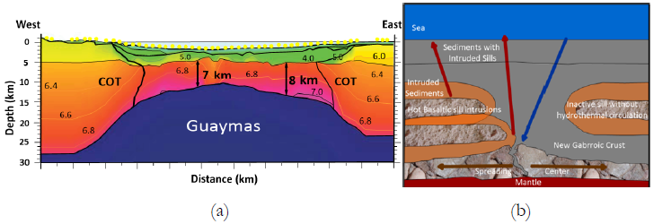
Figure 13 (a) Seismic velocity and crustal model for Guaymas extensional basin region of GoC, Mexico (modified after Lizarralde et al., 2007). (b) schematic diagram of subsurface basement, sills, sediments and arrow represent the liquid flow direction (modified after Teske et al., 2014).
For the surface layer (0-4 km), the low Q values contrast with one major patch (zone X in figures 11 and 12) of high Q value in the south-east zone of the region. The crustal structure obtained by Aragón-Arreola et al., (2005), Lizarralde et al., (2007) indicates that the south-central region of GoC, is masked by a thick layer of sill intruding the sediments deposited on the igneous layer. Thus, resulting in the low Q value and high attenuation in the surface layer. But the thickness of this sediment layer decrease from ~ 3 km in the Guyamas basin to the ~1.5 km in the Carmen basin. Thus, the presence of the igneous layer (Teske et al., (2014)) in the surface layer results in the increase of Q (zone X) in the south-east of the studied region, as shown in Figs. 11-12 at 1.0 Hz and 2.0 Hz. This feature does not show at the lower frequency (0.5 Hz) probably due to the small dimension of the high Q patch.
In the middle layer (4-8 km depth), two major patches (zones Y and Y1) of high Q value can be observed close to the ridge- transform system. First, the high Q patch Y at 0.5 and 1.0 Hz along the Guyamas basin increases with frequency from 53 at 0.5 Hz to 320 and 800 at 1.0 and 2.0 Hz, respectively. The subsurface representation of Guaymas basin shown in Fig. 13 suggest the presence of high heat flow due to intruded sills located along the western side of the spreading ridge. Thus, the cooler southwestern side has a higher Q value compared to the hotter northeastern side of the Guaymas Basin. The other high Q patch Y1 located along the Farallon Transform fault in a zone of high seismicity, where the rocks must be cool and rigid.
In the bottom Layer (8-12 km depth), a high Q value patch (Z) is observed along with the older and cooler continental crust. The obtained Q values in the depth range show a decreasing trend of Q towards the spreading ridges. This 8-12 km depth zone probably has a high flow of magma from the mantle near the ridge, as shown in Fig. 13, resulting in an increase of thermal flow in the bottom layer. Thus, low Q values and high S-wave attenuation takes place along the ridge transform fault system.
The obtained attenuation contours correlate with the crustal model proposed by Lizarralde et al., (2007) and Teske et al., (2014) and support the high attenuation of seismic energy observed along the gulf region. Also, the decrease in seismic velocity and high heat flow beneath the thin crust correlates with the high attenuation observed along the young plate boundary (Persaud et al., 2014; Teske et al., 2014; Vidales-Basurto et al., 2014; Lizarralde et al., 2007; Hasegawa 1985). These results also indicate that the seismic attenuation is decreasing towards the continental crust.
Bootstrap test
In order to inspect the stability of inverted Q structures, the bootstrap resampling scheme has been adopted. For the same, the initial population of 25 earthquakes has been divided into two subsets, with each subset having randomly selected 17 earthquakes. The inversion results for 1.0 Hz frequency are shown in Fig 14.
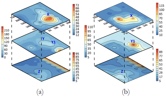
Figure 14 Bootstrap test results for two different subsets of initial population of earthquakes for depths (i) 0-4 km (ii) 4-8 km and (iii) 8 -12 km at 1 Hz frequency. The alphabets X, Y, Y1 and Z represents the identified low attenuation zones in different depth layers.
The comparison of bootstrap test results with Figs. 10-12, clearly reveal that for different subset of initial population of earthquakes, we are capable of detecting the same attenuation features on different depth layers. Thus, the resulted Q structure in this study is stable and consistent for different subset of original dataset. However, decreasing the number of earthquakes in bootstrap test has lowered the resolution of individual rectangular blocks, so few major differences in the attenuation structure has been observed in the bootstrap results.
A regional Q-frequency relation for this region has been prepared by using all 1944 estimates of shear wave quality factor at 18 different frequencies. Fig. 15 and 16 show the Q-frequency relation obtained using average values of Qs resulting from the inversion for each frequency. The best least square fit gives the relation Qs (f)= 20f1.2 for this region. Fig. 15 shows data used for obtaining this relationship. It has been observed that seismic Q strongly depends on the frequency f in the view of relation Q = Qo fn and increases with increase of frequency (Aki, 1980a). But this increase is not so widespread at low frequencies in comparison to high frequencies as we move from surface to depth (Kumar et al., 2015). Therefore, a relatively large error has been measured at high frequencies as shown in Fig. 15. Despite the large variation in Qs values at high frequencies, the resulted Qs values are providing the significant information for south-central GoC region.
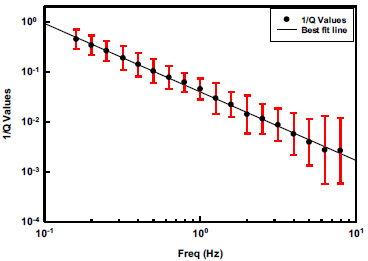
Figure 15 Frequency - dependent shear wave quality factor 1/Qs(f) relationship obtained from 1944 values of shear wave quality factor at different frequencies.
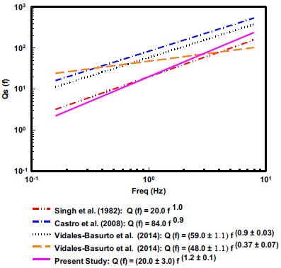
Figure 16 Comparison of obtained Q0-fn relation with other existing relations for the south-central GoC region.
The Qo-fn relation can be used to distinguish different regions into seismically active and stable areas. The parameters Qo and n represent heterogeneities and levels of tectonic activity, respectively (Kumar et al., 2015). Low values of Q0 < 200 indicate tectonically and seismically active regions, high values of Qo > 600 signify seismically stable regions, and intermediate values are expected in moderately active regions (Kumar et al., 2005). A correlation between the degree of frequency dependence and the level of tectonic activity in the area of measurement have been made by several researchers for a number of tectonic regions (e.g., Aki, 1980a; & Van Eck, 1988). They ascertained higher n values for tectonically active regions as compared to that of tectonically stable regions (Sharma et al., 2015). The obtained low Q0 =20 and high exponent n=1.2 of this relation indicate that the studied region is highly active with high attenuation. The resulted high value of n=1.2 is an artifact and can be considered as ~1.0. Similar, higher values of exponent n, has also observed for various highly active regions of world (Gupta et al., 1988, Akinci et al., 1994 & Vidales-Basurto et al., 2014).
We compare in Fig. 16, obtained relation with regional relationships obtained by previous studies in the GoC region using different techniques. It is seen that Q0-fn relation obtained with the estimates of Q from the inversion matches with other relations obtained for this region within the variability of the estimates shown in Fig. 15. The higher values of Q reported by Vidales-Basurto et al., (2014) are due to differences in the crustal volume sampled. Most of the paths sampled by them are outside the ridge zone and some includes the continental region. The estimates of Castro et al., (2008) correspond to the Mexican Basin and Range Provence, inside the continent. The estimates of Q from the Imperial Valley (Singh et al., 1982) are very similar to our estimates in south-central Gulf of California. These two regions have some geologic features in common, like the presence of sediments and high heat flow and explain the low values of Q obtained.
Conclusions
A frequency-dependent three-dimensional shear wave attenuation structure for the south-central Gulf of California, Mexico has been obtained using 98 records from 25 earthquakes recorded at six different stations. A total of shear wave attenuation structures at 18 frequencies has been obtained in this work that permitted us to identify zones of high and low attenuation that correlate well with geological and tectonic models of the region. The iterative inversion scheme used in this work gives results consistent with crustal models proposed by Lizarralde et al., (2007) and Teske et al., (2014) for the Gulf of California region. The average shear wave quality factor obtained from the different 108 blocks at different frequencies from inversion has been further used to develop the regional frequency dependent shear wave quality factor of form Qs (f) = 20 f1.2. The developed relationship has been compared with that available for this region. The comparison establishes the reliability of obtained shear wave quality factors in different blocks.

