


 nueva página del texto (beta)
 Inglés (pdf)
 Artículo en XML
 Referencias del artículo
 Enviar artículo por email
 Citado por SciELO
  Similares en
SciELO
Similares en
SciELO 
 Permalink
Introduction
Drylands cover 45% of the Earth’s surface (Prăvălie, 2016). Among one third of soils are moderately to heavily degraded due to erosion, loss of organic carbon, salinization, compaction, acidification and chemical pollution (FAO, 2015). Soil erosion is the issue that most affects Mexican agriculture (Cotler et al., 2006), which shows the lack of sustainable use of this natural resource.
Generally, the sowing of several agricultural products involves large tracts of land. The spatial variability observed in crops is a result of the complex interaction between edaphic (salinity, organic matter, texture, structure and nutrients), anthropogenic (soil compaction due to the traffic of farm equipment, irrigation and drainage and solute leaching), biological (pests and diseases), topographic (slope and altitude) and climatic (temperature, relative humidity and rainfall) factors (Ruiz-Garcia et al., 2009).
To evaluate the characteristics of agricultural soils, it is common to use a procedure for collecting soil samples to determine properties such as pH, nutrient composition and cation exchange capacity (CEC) from chemical and textural analyses. Indirect techniques such as Global Positioning System (GPS) or agricultural drones equipped with hyperspectral or RGB cameras are used to create normalized difference vegetation index (NDVI) or orthoimage maps. It is also useful to research the spatio-temporal variability causes of the factors that define productive efficiency and input optimization in an environmental sustainability framework (Loynachan et al., 1999), as well as to minimize the use of fertilizers and irrigation water, thus reducing the environmental impacts from agricultural activity (Robert, 2002). These techniques and procedures are known as Precision Farming (PF), useful to study and to mapping soil properties as reliable, fast and economical possible way.
Agricultural geophysics is an emerging discipline to obtain information about soil properties and conditions that influence the development of agriculture. They can be used to measure the impact of brackish wastewater use on a crop (De Carlo et al., 2020), monitor soil salinity (Aditama et al, 2017) and the dynamics of soil salts (Visconti and de Paz, 2016), groundwater exploitation, soil characterization considering salt concentration, safety inspection of embankments with leakage problems, detection of soil subsidence due to excessive pumping and tracking of groundwater aquifer contamination by leachate (Song and Cho, 2018). Similarly, other research suggests using geophysical methods to map soil behavior by relating electrical conductivity to crop yield (Fano, 2019), information that could have wide application in identifying contamination, sampling soils, and deriving input recipes for nutrients, seeds, and herbicides (Lech, et al., 2016). With the different techniques that can be employed from geophysics, it allows for improved sustainable management of agricultural land because the information generated in terms of salinity, soil texture, soil moisture, cation exchange capacity (Sadatcharam, 2019), nutrients, sediments and water can be used in farmers' decision-making (Heil and Schmidhalter, 2017, and Ameglio, 2018).
The two groups of geophysical methods that are highly used for agricultural purposes are electrical (Electrical Resistivity Tomography, Electrical Profiling) and electromagnetic (EM Profiling and GPR) techniques. These methods demonstrate their effectiveness and economic benefits in the implementation of PF (Corwin and Lesch, 2003) when determining the boundaries between genetic types of soils (Pascual et al., 1995) and changes in soil salinity (Rhoades and Corwin, 1981, Williams and Baker, 1982) or moisture (Edlefsen and Anderson, 1941, Kirkham and Taylor, 1950, McKenzie et al., 1989); whereas magnetic, spontaneous potential and seismic refraction are methods less frequently applied for agriculture soil studies (Allred, 2009).
To propose a conductivity model for unconsolidated rocks, the Ryjov’s algorithm was developed for both the geometrical microstructure and electrochemical process for wide ranges of water salinity and clay concentrations. The forward petrophysical problem consists of the calculation of rock resistivity values on the base of properties of unconsolidated sediment (mixture of sand and clay). The inverse problem consists of the estimation of the properties’ clay content, porosity and CEC on the base of soil resistivity and pore water salinity, taking into account the soil petrophysical model of the site (Ryjov and Shevnin, 2002). Subsequently, a new methodology applied to environmental impact studies of the oil industry in Mexico (Delgado-Rodríguez et al., 2018) was developed, including geoelectrical survey and electrical measurements in soil and groundwater samples (Shevnin et al., 2006a, b). This methodology, using Ryjov's algorithm, resulted in the mapping of the aforementioned petrophysical parameters for accurate delineation of the hydrocarbon contamination plumes (Shevnin et al., 2004).
The first application of this procedure in soil studies was performed by Delgado-Rodríguez et al. (2012) in a small plot (800 m2) of sandy-loam soils located in the surroundings of Oaxaca city, Mexico, where clay, porosity and CEC maps were determined from electrical data obtained from a lab and Electrical Resistivity Tomography (ERT) survey. A linear regression analysis showed a good correlation (R2 = 0.93) between clay content values determined from Bouyoucos textural analysis and clay content values obtained from electrical measurements in lab. However, soil sampling, which is needed for electrical measurements in the laboratory, is invasive and the results obtained in the area were very timely. Furthermore, a regular correlation (R2 = 0.7) between clay content values determined from the ERT survey and from the Bouyoucos textural analysis was shown. The application of the ERT method is not invasive, but it is inefficient for application on expansive agricultural land.
As a second case, the electrical survey was performed on a small farm near to Guasave city, Sinaloa, Mexico, where a wide variety of soil textures (clay, silty clay, clay loam, loam, sandy loam, silt loam, sandy clay loam, and silt clay loam) were observed (Gastélum-Contreras et al., 2017). In this case, electrical profiling (EP) was used as a technique faster than the ERT method. Textural analyses were carried out on 30 soil samples collected at points where EP measurements were taken. Fines (clay + silt) content values were comparable (R2 = 0.91) to those obtained based on apparent resistivity values and Ryjov's algorithm, providing reliability to the maps obtained for fines content and porosity.
This paper presents the results of the joint processing of apparent resistivity from an EP survey, soil salinity and moisture values collected in three plots located in the state of San Luis Potosí (SLP), Mexico (Figure 1). The agriculture plots are located in the municipality of Villa de Arriaga, 60 km southwest of the city of San Luis Potosí, SLP, Mexico, at an average height of 2,160 m.a.s.l., where Durisols (Figure 1) type soils predominate. Every year, in the three agricultural plots, A, B and C with 9.6, 6.8 and 4.2 ha, respectively, the same barley sowing technique is applied, neither fertilizers nor irrigation systems (seasonal crops) are used. The results obtained from each plot (fines content, moisture, salinity, porosity, CEC and K maps) were compared with textural, crop yields and fertility data. A short ERT profile was performed in a plot help to visualize the soil thickness from a 2D resistivity cross-section and, therefore, to define the optimal study depth for an EP survey.

Materials and Methods
1.1. Theoretical Soil Model of Ryjov
A model that includes components of unconsolidated sediments and electrochemical resistivity estimation of pore-water, resulting in the estimation of the rock resistivity, was presented for the first time by Ryjov and Sudoplatov (1990). Solid grains of sand and clay make up an insulating skeleton where their capillaries are seen as hollow cylinders with different radii. The sand component contains a wide cylindrical porous system which are much larger than the thickness of the electrical double layer (EDL). The micropores of the fines component are very narrow, which is close to the thickness of the EDL. The thickness of the EDL depends on the water salinity and increases with decreasing salt concentration. At near-surface conditions, when the salt concentration changes from 0.02 to 2 g/l, the thickness of the EDL oscillates within the range of 0.3 - 3×10⁻⁸ m. The total volume of pores for sand and fines is taken into account separately through the value of its porosity, therefore the model of the mixture consists of two types of capillaries with different radii (Shevnin et al., 2007). The capillaries of sand and clay can be connected in series, parallel or a combination of both. In order to include the influence of the pore microstructure in the model, we have taken into account the tortuosity of the sand pores as a function of the content of solid sand grains in the mixture.
The conductivities of the sand (σsand) and fines (σfines) components can be calculate using:
where σsandcap and σfinescap are the conductivities of sand and fines (fines + silt) capillaries, respectively, and φsand and φfines are the porosities of the sand and fines components, expressed as volume fractions of the total volume. In the pore system of the sand, which has wide capillaries, the average conductivity of sand channels σsandcap does not depend on the capillary radius and corresponds to the free-water conductivity σw (electrolytic conductivity).
The conductivity of water solutions, with and without the influence of capillary walls, depends on salt concentration, anion and cation properties, as well as the influence of the EDL.
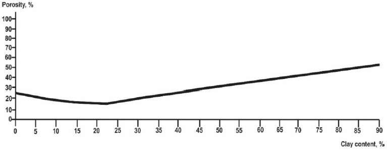
The structure of clayed soils is described using an ideal packing concept for binary mixtures of clay and bigger spherical particles (McGeary, 1961). According to this model (Figure 2), while the clay content is less than the sand porosity, the fines particles, which have an average radius much smaller than sand grains, fit within the sand pores. When the clay fraction exceeds the sand porosity, the sand grains become suspended in the clay host (Shevnin et al., 2017). Figure 2 shows the theoretical dependence of porosity from clay content for model A. The porosity curve begins at 25% (sand porosity), reaching a minimum when clay content is equal to sand porosity and all sand pores are filled with clay, then increases until clay porosity (55%). The left part of the curve was formed under the influence of sand porosity, while the right part is influenced by clay content and clay porosity.
The total porosity φt of the soil can be determined by the following equations (Marion et al., 1992, Revil et al., 2002):
where Cfines is the volumetric fines content (clay + silt) in a sand-fines mixture.
When Cfines > φsand, the total soil conductivity, σt, is equal to the conductivity of the fines component (σfinescap), fines porosity and salt concentration. The sand component can only have an influence by decreasing the volume of the fines host (Cfines):
When Cfines < φsand, σt it is defined by both the φsand and φfines, which is saturated by the pore-water of a given salinity.
The interconnections of pore systems can be connected in parallel or in series. In case of capillaries connected in parallel, σt is simplified to:
where σprl is a conductivity of a soil fraction consisting of a sand-fines mixture and the parallel connections of capillaries.
In case of capillaries connected in parallel, σt is simplified to:
In soils, the presence of both parallel and series capillaries is common. Some part of the fines is smeared on the sand’s pore walls, while other parts of fines is found inside the sand pores as plugs. Capillaries are split into a volumetric part of parallel capillaries equal to M and a serial part equal to 1 − M. Now, it is possible to calculate the σt according to:
An example of solution of the forward problem using equations (5) and (8) is shown in Figure 3 considering soil properties similar to those presented in Figure 2, where theoretical soil resistivity (or its inverse, conductivity) curves versus pore-water salinity are observed. Pore-water salinity is calculated for the following parameters: NaCl solution and soil saturation, temperature 20°C, sand porosity 25%, fines porosity 55%, the CEC of clay 40 cmol (+) / Kg (~3 g/l). The values on the curves indicate fines (in this case, only clay) content from sand (0%) up to 100% fines and soil porosity as a percentage (Figure 3). Note that for high pore-water salinity (> 10 g/l) the soil resistivity curves are situated above and practically in parallel to the pore-water resistivity curve, which is similar to the sand curve (electrolytic conductivity effect). At lower pore-water salinity, the soil resistivity curves for different fines-sand mixtures are situated below and not parallel to the pore-water curve due to the influence of the EDL (superficial conductivity effect). The dashed of the blue line represents pore-water resistivity (Figure 3). This model is described in detail by Shevnin et al. (2017).
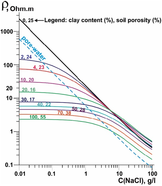
Figure 3 Theoretical dependence of the resistivity of a sandy-clay mixture on groundwater salinity. Clay porosity = 55%, sand porosity = 25%. Modified from Shevnin et al. (2017).
1.2. Estimation of Soil Properties
Considering this model using equations (5) and (8), it is possible to generate theoretical curves of electrical resistivity from any soil consisting of sand and fines (clay and/or silt) versus pore water salinity (solution of the forward problem, Figure 3) from defined parameters: fines content, porosity, and CEC.
The difference between the experimental (ρexp) and calculated resistivity (ρcal) curves is minimizing by the standard Root Mean Square (RMS) error. RMS error is the standard deviation of the prediction errors or residuals. Residuals are the difference between the ρexp and the ρcal values. RMS is calculated for n pairs of values of ρexp and ρcal, using the following equation:
Using the PetroWin program developed by Ryjov (Ryjov and Shevnin, 2002), an iterative inversion process of minimizing of the RMS error between the experimental (from electrical measurements in lab) and theoretical (theoretical model above described) curves is made. Different parameters can be modified during the iterative inversion process, such as pore-water salinity (including types of anions and cations with their valence, hydration number, sorption constant and mobility), porosity, capillary radii, moisture and cementation exponent for each fines and sand components of the soil, as well as the CEC for fines component and the temperature of the soil. Finally, calculation of fines content, porosity and CEC values for the soil sample is performed as the solution of the inverse problem.
a) Determination of Soil Salinity by the Saturation Extract Method
Soil salinity was determined by the saturation extract method (USSLS, 1954), whose procedure is as follows: first, an approximately 2/3 if a beaker is filled with dried and sieved soil. De-ionized water is added to the soil in the beaker while stirring with a spatula until reaching saturation level. The soil paste must glisten, flow slightly when the container is tipped, slide cleanly from the spatula, and readily consolidate after a trench is formed upon jarring the container. After mixing, the samples should rest at least four hours, then the free water is removed. The saturated paste is transferred to a Buchner funnel using filter paper where the pore-water is extracted by a vacuum environment. Subsequently, the electrical conductivity (EC), and therefore the salinity of the extract is determined using a conductivity meter for a reference temperature of 20 oC (Miller and Curtin, 2007).
According to the EC values of the extract, there are no salinity problems in the 19 collected soil samples within EC range of 0.150 and 0.575 dS/m (Table 1). According to the Agriculture Department of the United States of America (Staff Soil Survey Division Agriculture, 1993), it is classified as non-saline soil and corresponds to salinities in the range 0.10 - 0.35 g/l with a mean value of 0.21 g/l.
b) ERT Method
The application of the ERT method is based on an apparent resistivity determination supported by the linear array (e.g. Dipole-Dipole, Wenner-Schlumberger) of many electrodes emplaced with a constant interval and connected to a resistivity meter. ERT is applied to obtain a geoelectrical image of the sub-surface using electrical measurements made on surface along profile. Such profile measurements allow a two-dimensional (2D) interpretation (interpreted section) using the Res2DInv software (Loke and Barker, 1996).
During the ERT survey, direct current (I) is injected into the soil and subsoil through a pair of electrodes commonly named A and B. The potential difference (∆V) is measured by a pair electrodes M and N. The electrical field is distributed into a volume of soil whose size can be estimated from the distance between the AMNB electrodes (Keller and Frischknecht, 1966), thereby obtaining a value of ρa for each measurement point using:
Where:
ρa is the apparent resistivity (Ohm.m), K is a geometric factor (m), ∆V is the potential difference measured (mV), I is the current intensity (mA), and R is the resistance (Ohm). K depends on the array geometry and can be calculated using equation (11), where rAM, rBM, rAN and rBN are the separation distances between electrodes A - M, B - M, A - N and B -N, respectively. The ρa value is a bulk resistivity of soils and rocks influencing the flow current.
An ERT profile of 38.4 m in length was carried out on agricultural plot A (Figure 4A) to obtain a geoelectrical image of the soil and subsoil using a Wenner-Schlumberger array with a constant electrode spacing of 0.2 m and AB/2 selected from 0.3 to 2.1 m, thus enabling a detailed shallow study up to a depth of 1 m. The separation between sounding points was 0.6 m with a total of 65 measurement points. A Saturn GEO Earth Ground Tester produced by LEM Norma GmbH, Austria (Fluke Corp., 2005) (Figure 4B) with a sensitivity of 1 mOhm and a maximal current of 50 mA at 128 Hz was used to obtain electrical resistance (R) measurements and calculate the resistivity values from equations (10 and 11).
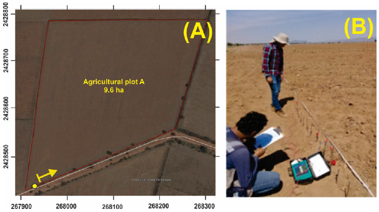
Figure 4 ERT survey. (A) Location of the ERT profile (yellow arrow) at the SW end of plot A. The yellow circle indicates the location of the excavation and soil profile. (B) ERT measurements using a Saturn Geo Earth Tester.
Res2DInv software (Loke and Barker, 1996) was used for performed the inversion of the experimental data (ρa cross-section), providing a soil resistivity (ρ) cross-section. Res2DInv software use the smoothness-constrained least-squares method inversion technique, which can be optimized to achieve successful results in both areas where the subsurface resistivity varies in a smooth manner and areas with sharp boundaries. The ρ cross-section has the same number of layers with same the thicknesses along profile (Loke and Barker, 1996), having the advantage of separating resistivity values for a single layer, e.g. topsoil.
A soil profile could be easily observed through excavation works in a canal near the southern limit of plot A (Figure 5A). The hole of approximately 1 m deep exposed three horizons: horizon A as topsoil, horizon B subsoil composed of sand-clay-silty material, and horizon C given by fragmented and weathered limestone as parent material (Figure 5A).
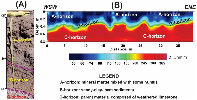
Figure 5 ERT results. (A) Soil profile with three horizons and their thickness observed in excavation near to ERT profile. (B) Interpreted 2D resistivity model from ERT data where three soil horizons are differentiated.
The ERT profile was initiated 20 m ENE from the excavation (Figure 6A) and the inversion model is shown in Figure 5B, where three resistivity domains are clearly observed in correspondence with the soil profile (Figure 5A). A first and superficial conductive layer (ρ ≤ 85 Ohm.m) given by the topsoil (soil + organic matter), followed by a layer of intermediate resistivity values (85 < ρ ≤ 120 Ohm.m) given by subsoil, and finally a resistive basement (ρ > 200 Ohm.m) due to the presence of carbonate rocks are observed in Figure 5B.
c) EP Method
One of the geoelectrical methods widely used in near surface studies is EP. The EP method is commonly used to study aquifers and rock properties (Ucha et al., 1984), to support archaeological surveys (Perdomo, 2013), geotechnical studies (Adebisi et al., 2016), geological mapping, and the detection of fractures (Demirel et al., 2018). The principle of the method consists of performing resistivity measurements through a four-electrode array AMNB, similar to the one used in the ERT survey, along a line or profile on the surface. The EP array is moved along the profile, obtaining only one ρa value per measurement point, thereby keeping the mutual distances between electrodes unchanged. The values of ρa obtained represent the lateral changes of electrical resistivity for a constant study depth.
The application of EP is faster than the ERT method. The EP method, while it does not provide detailed lithological information (layers and their thickness), is able to detect horizontal changes in soil resistivity for specific study depths in a short time.
In this work, an EP survey was conducted using the Saturn GEO Earth Ground Tester (Fluke Corp., 2005) with a Wenner array for a = 0.5 m, guaranteeing study depths of ~ 0.25 m (Banerjee and Pal, 1986). Although EP only provides ρa, according to the soil thickness observed in the canal and ERT section, we consider that the ρa values obtained from EP for a study depth of 0.25 m would be comparable to the true resistivity of topsoil.
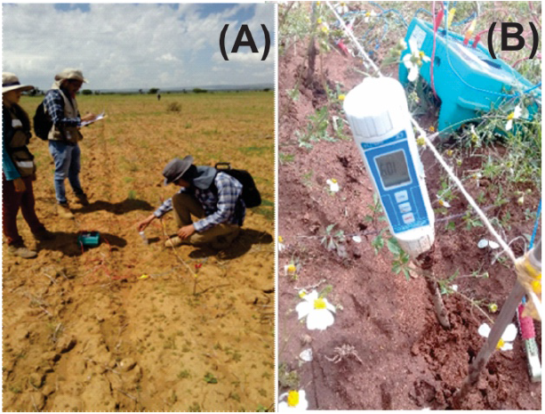
Soil moisture measurements using a Lutron PMS-714 meter with a 0.2 m stainless steel probe were obtained in situ at each EP measurement point (Figures 6A and 6B), therefore, 341 ρa and soil moisture measurements were distributed in 30 parallel profiles.
The ρa range (Figure 7) should be strongly controlled by the variation of its moisture (Figure 8), as seems to be the case for plot B, where the predominance of high values of apparent resistivity (Figure 7B), which correlate with the minimum moisture values (Figure 8B), this correlation not being so evident in plots A and C (Figs. 7A, 7C, 8A and 8C). Note the low moisture range (5% -17%) in all plots (Figure 8) due to there being no irrigation system in the study area and the EP survey being carried out during the dry season. The maximum moisture values (15%-17%) are concentrated at the southern end of plot A (Figure 8A) where occasionally the excavation and leveling process of the canal includes pouring water on the ground. Therefore, we believe that other factors such as texture or organic matter content control the variability of the apparent resistivity.
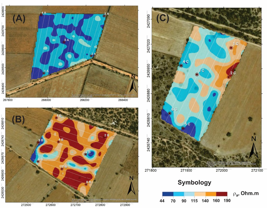
Figure 7 Apparent resistivity maps for agricultural plots A, B and C. Red dots represent the soil sampling locations.

4.1. Soil Sampling and Electrical Measurements in Laboratory
A total of 19 random soil samples for the depth interval 0 - 0.3 m were collected and exposed to a drying and homogenization process, the soil sample being well stirred. For the selection of sampling points, the resulting apparent resistivity and soil moisture maps were considered (Figures 7 and 8).
Each of the soil samples, after being dried and homogenized, were divided into five similar soil boxes, water with a certain salinity was then added (different for each soil box, ranging between 0.1 and 70 g/l) so that the sample was saturated (Figure 9A). The soil box was a rectangular plastic container. Two electrodes, A and B, were placed on each of the smaller sides of the container to inject current I into the soil from the resistivity meter. Two potential measuring electrodes (M and N) were placed on the larger side of the container to obtain potential difference (∆U) measurements. The measurements were recorded by the Saturn Geo Earth Ground Tester (Fluke Corp., 2005, Figure 9B).
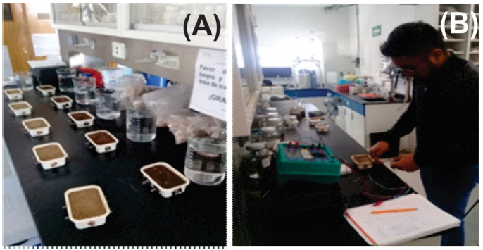
Figure 9 Electrical measurements of soil samples in laboratory. (A) Soil sample placement process in five resistivity boxes, (B) Taking of soil resistivity measurements using the Saturn Geo Earth Ground Tester.
The soil resistivity (ρ) value in each soil box was determined by the expression:
where A is a calibration factor that includes the shape of the soil box and the position of the electrodes.
Soil resistivity depends on temperature. For the correction of resistivity measurements to 20°C the following simple formula was used:
Where: Tm = Temperature of saturated soil (°C), ρ(Τm) = saturated soil resistivity at temperature Tm, ρ(20) saturated soil resistivity corrected at 20 °C, α is a coefficient equal to 0.0177 1/°C (Beklemishev, 1963).
At the end of the measuring process, there were five pairs of values (one for each soil box) of soil resistivity and water salinity, resulting in an experimental soil resistivity vs pore water salinity curve corresponding to each soil sample. To estimate the soil properties, we minimize the difference between the experimentally and calculated resistivity curves defined by the standard RMS fitting error, using an iterative inversion process briefly described in section 2.1.2.
Table 1 shows the modeling results of the 19 soil samples collected in the three plots, including the RMS error between calculated and theoretical curves for each soil sample.
Table 1 Soil properties in soil samples obtained from EP survey and Ryjov’s algorithm.
| No. | Sample | X | Y | Fines (%) |
Porosity (%) |
CEC (cmol (+)/Kg) |
K (cm/h) |
EC dS/m) |
RMS error |
|---|---|---|---|---|---|---|---|---|---|
| 1 | 1A | 267980 | 2428471 | 41 | 26.7 | 3.60 | 0.17 | 0.196 | 2.3 |
| 2 | 2A | 268227 | 2428561 | 41 | 26.7 | 0.40 | 0.17 | 0.189 | 3.0 |
| 3 | 3A | 268294 | 2428770 | 40 | 24.0 | 3.50 | 0.18 | 0.25 | 4.8 |
| 4 | 4A | 267967 | 2428775 | 45 | 26.6 | 0.04 | 0.14 | 0.15 | 5.0 |
| 5 | 5A | 268085 | 2428634 | 45 | 26.1 | 4.38 | 0.14 | 0.242 | 4.6 |
| 6 | 1B | 272617 | 2426827 | 40 | 26.0 | 1.95 | 0.18 | 0.216 | 4.9 |
| 7 | 2B | 272810 | 2426748 | 48 | 30.2 | 7.00 | 0.13 | 0.267 | 2.4 |
| 8 | 3B | 272735 | 2426679 | 44 | 27.7 | 0.39 | 0.15 | 0.156 | 4.9 |
| 9 | 4B | 272625 | 2426729 | 42 | 29.4 | 20.83 | 0.16 | 0.553 | 3.2 |
| 10 | 5B | 272544 | 2426727 | 41 | 28.7 | 29.98 | 0.17 | 0.648 | 3.0 |
| 11 | 6B | 272543 | 2426650 | 44 | 27.7 | 6.42 | 0.15 | 0.21 | 3.9 |
| 12 | 7B | 272639 | 2426620 | 39 | 27.3 | 37.96 | 0.19 | 0.993 | 4.3 |
| 13 | 8B | 272737 | 2426557 | 40 | 28.0 | 5.84 | 0.18 | 0.307 | 2.4 |
| 14 | 1C | 272021 | 2427010 | 50 | 32.5 | 38.93 | 0.12 | 0.748 | 2.4 |
| 15 | 2C | 272014 | 2426927 | 43 | 30.1 | 6.23 | 0.16 | 0.334 | 4.8 |
| 16 | 3C | 271925 | 2426934 | 55 | 36.9 | 32.12 | 0.1 | 0.653 | 2.6 |
| 17 | 4C | 271880 | 2426959 | 59 | 40.1 | 25.79 | 0.08 | 0.487 | 3.2 |
| 18 | 5C | 271885 | 2426782 | 67 | 38.9 | 46.33 | 0.07 | 0.676 | 0.7 |
| 19 | 6C | 271848 | 2426824 | 62 | 39.1 | 39.23 | 0.08 | 0.637 | 2.5 |
The hydraulic conductivity (K) was calculated based on the fines content using two empirical formulas:
where K is the saturated soil hydraulic conductivity (m/day) and C is the fines content in the interval 0 - 1. The restrictions are the following: the fines content cannot be zero, and it is only valid for unconsolidated formations.
The equation (14) was proposed by (Shevnin et al., 2006b) for soils with a clay content ≥ 35% (e.g. clay loam soils). However, in silt and silt-loam soils, when the clay content < 35 % (e.g. loam, sandy loam and sandy clay loam), it is more reliable to use equation (15) proposed by Delgado-Rodríguez et al. (2010). Both equations showed good correlation with the results achieved using a falling head permeameter (Delgado-Rodríguez et al., 2010). The calculated K (m/day) values were converted to K (cm/h) values (see Table 1).
4.2. Estimation of Soil Properties Based on Electrical Measurements Obtained in Fieldwork
By using the same algorithm modelling, apparent resistivity and soil moisture values obtained from EP survey, as well as soil salinity values, it is then possible to determine, fines content, porosity, CEC and K maps for each agriculture plot. It is necessary to have an initial model based on theoretical models determined in representative soil samples in the laboratory. In addition, soil moisture and salinity maps are shown.
4.3. Textural Analysis of Bouyoucos
Knowledge of soil texture is important because it affects soil fertility and determines the amount of consumption and water storage in soil. The relative proportion of sand, silt and clay in a soil can be used to determine a texture calculated from the density of an aqueous soil suspension measured by hydrometer following the Bouyoucos procedure (Bouyoucos, 1962).
The procedure consists of separating aggregates and analyzing particles. A measured time is chosen for the separation of larger particles and for smaller ones. Generally, after 40 seconds the sand particles (diameter greater than 0.005 mm) settle at the bottom of the hydrometer, while silt particles (diameter greater than 0.002 mm) need 2 hours. In the case of clay, up to 24 hours are required for an accurate calculation of settled particles. By knowing the length of the hydrometer, we can calculate the velocity of the particles and their diameters, and thus determine the sand, silt and clay contents.
The results of the textural analysis of Bouyoucos carried out on the 19 soil samples are shown in Table 2. Table 2 shows that soil sandy clay loam is predominant, especially in plots A and B, that is, sand > 45%, silt < 28% and clay content > 20%. In plot C, the soils show a slight increase in clay content.
Table 2 Texture analysis results in 19 soil samples
| Plot | Soil sample | X | Y | Sand, % | Silt, % | Clay, % | Texture |
|---|---|---|---|---|---|---|---|
| A | 1A | 267980 | 2428471 | 68.2 | 16.0 | 15.8 | Sandy loam |
| 2A | 268227 | 2428561 | 59.3 | 20.0 | 20.7 | Sandy clay loam | |
| 3A | 268294 | 2428770 | 57.3 | 20.0 | 22.7 | Sandy clay loam | |
| 4A | 267967 | 2428775 | 49.3 | 22.0 | 28.7 | Sandy clay loam | |
| 5A | 268085 | 2428634 | 53.3 | 22.0 | 24.7 | Sandy clay loam | |
| B | 1B | 272617 | 2426827 | 59.3 | 16.0 | 24.7 | Sandy clay loam |
| 2B | 272810 | 2426748 | 51.3 | 24.0 | 24.7 | Sandy clay loam | |
| 3B | 272735 | 2426679 | 55.3 | 19.3 | 25.4 | Sandy clay loam | |
| 4B | 272625 | 2426729 | 57.3 | 21.3 | 21.4 | Sandy clay loam | |
| 5B | 272544 | 2426727 | 59.3 | 23.3 | 17.4 | Sandy loam | |
| 6B | 272543 | 2426650 | 55.3 | 19.3 | 25.4 | Sandy clay loam | |
| 7B | 272639 | 2426620 | 61.3 | 19.3 | 19.4 | Sandy loam | |
| 8B | 272737 | 2426657 | 59.3 | 17.3 | 23.4 | Sandy clay loam | |
| C | 1C | 272021 | 2427010 | 50.0 | 25.3 | 24.7 | Sandy clay loam |
| 2C | 272014 | 2426927 | 56.0 | 21.3 | 22.7 | Sandy clay loam | |
| 3C | 271925 | 2426934 | 44.0 | 25.3 | 30.7 | Clay loam | |
| 4C | 271880 | 2426959 | 40.0 | 33.3 | 26.7 | Loam | |
| 5C | 271885 | 2426782 | 31.3 | 32.0 | 36.7 | Clay loam | |
| 6C | 271848 | 2426824 | 37.3 | 32.0 | 30.7 | Clay loam |
Results and Discussion
Soil properties maps obtained from electrical measurements in the laboratory and infield using the Petrowin software (algorithm of Ryjov) were analyzed and compared with soil textural and fertility results, as well as crop yield per planted hectare.
1 Comparative Analysis of Fines Content Values Determined in the Laboratory
Silt and clay contents were determined in 19 collected soils samples using Bouyoucos textural analysis, whose sum represents the fines content. The fines contents were also determined in the same soil samples based on electrical measurements taken in the laboratory using the PetroWin program (Ryjov’s algorithm). Both results are shown in the comparative chart in Figure 10, where a low dispersion around the function Y = X (R2 = 0.94) can be observed, giving reliability to the calculation process for soil properties from electrical measurements in the laboratory. Only the 1A and 4A samples show some differences between both results. Furthermore, the Bouyoucos method includes, prior to particle analysis, the elimination of organic matter in soil, while for electrical measurements conducted in the laboratory the soil sample should only be homogenized, thereby maintaining its organic matter, which is considered in the calculation of the CEC.

2 Soil Properties Sections from ERT Profile
The resistivity section interpreted, along with the soil moisture and salinity information, was recalculated in the fines content, porosity, K and CEC sections.
The fines content section (Figure 11A) shows higher values of fines content in topsoil soil, reaching values greater than 50%, while the carbonated basement (parent matter) contains fine content less than 16%. The porosity of the topsoil (Figure 11B) displays high variability into 21 to 45% interval. Ryjov’s algorithm calculates soil porosity as a function of fines content (Shevnin et al., 2007). According to Ryjov’s theoretical soil model (see Figure 2), when the fines content (clay + silt) is less than the sand porosity (mean sand porosity is 28%), the fine particles occupy the sand pores, resulting in a decrease of the soil porosity. If fines content is greater than sand porosity (fines content > 60%, Figure 12A), soil porosity increases (porosity > 45%, Figure 11B).
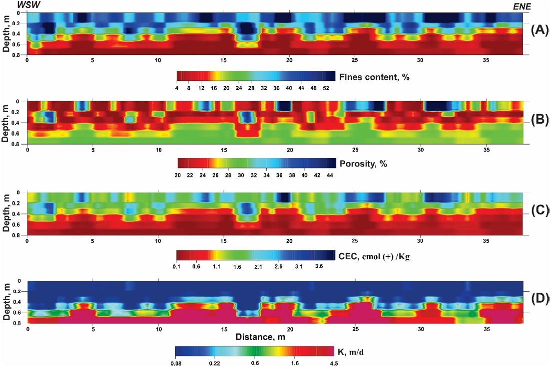
Figure 11 Soil properties section. (A) Electrical resistivity, (B) Porosity, (C) CEC and (D) Hydraulic Conductivity.
The hydraulic conductivity (Figure 11C) shows K values less than 0.3 m/day at a depth between 0 and 0.3 m, coinciding with highest fines content values (Figure 11A). A stronger contrast is shown at depths greater than 0.60 m, where K > 5 m/day, indicate the presence of a permeable carbonated substrate.
In general, the section of Figure 11D indicates low CEC values. Low CEC values in the topsoil (1.3 to 4.6 cmol (+) / Kg) may be due to both texture and organic matter content. In the case of texture, the predominant soil in the studied plots is sandy-clay-loam, where the clay content is less than 25%. Besides, the modeling process for soil resistivity vs. salinity curves using the PetroWin program shows low CEC values, which could mean that the clay present in soils from the studied plots is of the kaolinite type. On the other hand, during the Bouyoucos textural analysis, most soil samples showed low organic matter content during their destruction process using hydrogen peroxide. Furthermore, CEC values < 0.7 cmol (+) / Kg clearly show the carbonated rock (Figure 11D).
The application of the ERT method has the advantage of being able to show three soil horizons and their thicknesses in detail (horizons A, B and C, Figure 5B). However, ERT is not an efficient method to characterize large areas such as agricultural plots, it being necessary to use faster electrical or electromagnetic methods such as EP.
3 Soil Maps Based on Electrical Measurements
The apparent resistivity (from the EP survey), soil moisture, and salinity values were processed using the PetroWin software, results in fines content, porosity, K, and CEC maps. The fines content maps for each plot are shown in Figure 12, where the location of the soil sampling points is indicated. In general, fines content maps show great variability. In plot A (Figure 12A) soils with higher percentages of fines content (36-48%) predominate, while in plot B (Figure 12B) the lowest determined values predominate (11-24%), leaving plot C in the middle (17-30%) (Figure 12C).
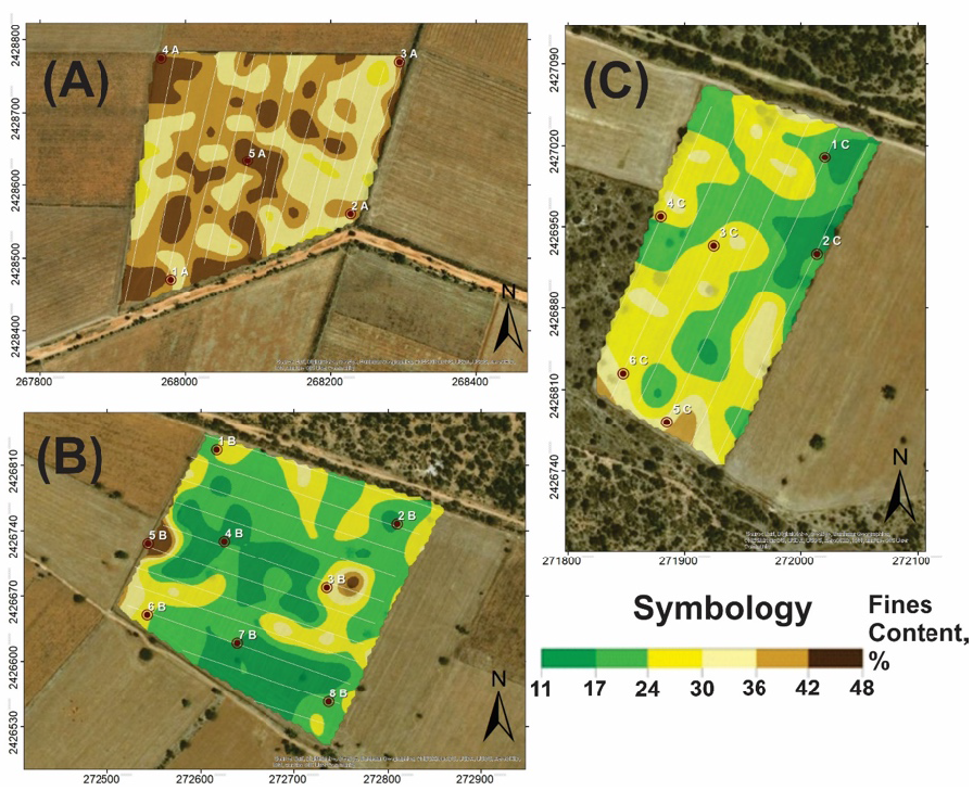
Figure 12 Fines content maps of soil for agricultural plots A, B and C. Red dots represent the soil sampling locations.
The soil porosity maps for the three agricultural plots (Figure 14) show moderately porous to highly porous soils (Pagliai, 1988) with a porosity interval between 20% and 32%. Plot A has the highest porosity values (Figure 13A) in correspondence with the highest content of fines (Figure 12A), while plots B and C show lower values. The aforementioned relationship between fines content and porosity has the same effect on the fines content (Figure 11A) and porosity (Figure 11B) sections as results of the application of the ERT method.
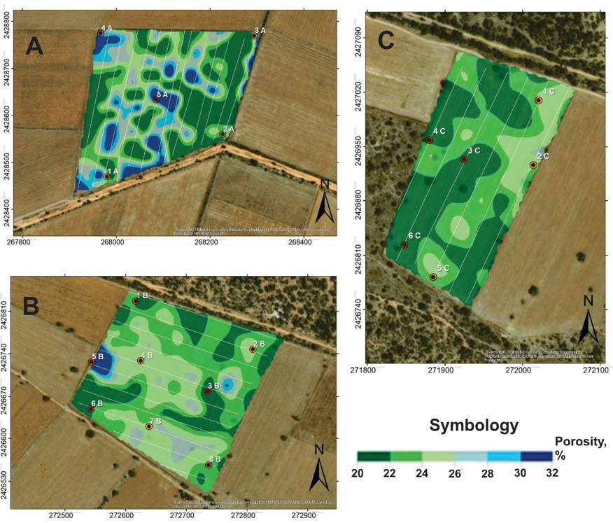
Figure 13 Porosity maps of soil for agricultural plots A, B and C. Red dots represent the soil sampling locations.
The soil hydraulic conductivity (Figure 14) is related to the fines content (see equations 14 and 15) determined using the PetroWin software. According to the permeability classification of the agricultural soil (Bendixen et al., 1948), the three plots are classified from very slow to moderate. Plot A (Figure 14A) has a very slow to slow permeability with K values less than 0.5 cm/hr. Plots B (Figure 14B) and C (Figure 14C) show a predominance of moderately slow soils with K values being more variable in plot B than plot C, with some areas reaching extreme values of very slow to moderate permeability.
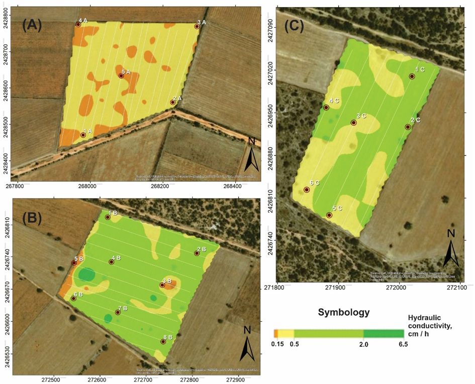
Figure 14 Hydraulic conductivity (K) maps of soil for agricultural plots A, B and C. The K color scale was designed by taking into account the permeability classification (Bendixen et al., 1948). Red dots represent the soil sampling locations.
A representative soil sample was prepared using soil samples collected in each plot. For example, in plot A a bulk sample A of 7.55 kg was formed as a result of the sum of five samples (1A to 5A) of ~ 1.5 kg each. Sample A was homogenized and, subsequently, the quartering method (Campos and Campos, 2017) was applied to obtain a representative soil sample: first, the sample A is divided into quarters, whereupon two opposite quarters are discarded, then the remaining two quarters are homogenized, flattened, then finally divided into quarters, the two opposite quarters being discarded again. The process was repeated once again resulting in a homogenized sample of ~ 1 kg representing plot A. The same process is performed for plots B and C, respectively.
CEC is related to clay and organic matter contents in soils. CEC values for soil representative samples were determined in the laboratory using the ammonium acetate saturation method (CECAAM) (Kitsopoulos, 1999), resulting in 5.79 cmol (+) / Kg, 7.02 cmol (+) / Kg and 9.25 cmol (+) / Kg for plots A, B and C, respectively.
In January 2019, the barley crop yields were obtained in each plot. Markedly low productivity was observed in plot A (1600 kg/ha), meanwhile plots B (2400 kg/ha) and C (2600 kg/ha) showed similar levels of production (Figure 16). These crop yields correlate with the above-mentioned CEC values. A higher harvest yield corresponds to higher CECAAM values (Figure 15A). The three plots are close to each other, unfertilized, and where the same sowing technique (in rainy season) was used without an irrigation system. Therefore, the availability of cations and nutrients was proportional to the crop yield.
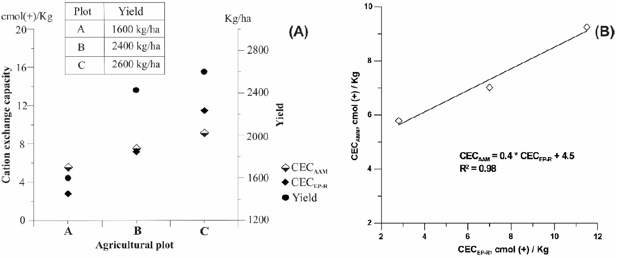
Figure 15 Comparative analysis of CEC values determined in soil representative samples. (A) Relationship between CEC and crop yield in agricultural plots A, B and C. (B) Linear correlation graph between CEC values determined using the CECAAM and CECEP-R methods. CECAAM = CEC determined from the ammonium acetate method, CECEP-R = CEC determined from EP survey and Ryjov’s algorithm, Yield = barley crop yields.
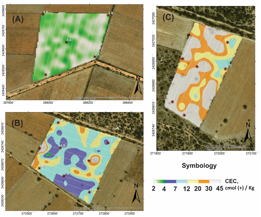
Figure 16 CEC maps of soil in agricultural plots A, B and C. Red dots represent the soil sampling locations.
Figure 16 shows the CEC maps determined from the EP survey and Ryjov’s algorithm for the three agricultural plots. In general, the CEC maps show low values for the three plots, however, it can be clearly observed that plot A (Figure 17A) has the lowest CEC values (CEC < 3.8 cmol (+) / Kg and mean CEC = 2.8 cmol (+) / Kg). In plot B (Figure 17B), the CEC values are in the range 3.8 - 45 cmol (+) / Kg (mean CEC = 7 cmol (+) / Kg). Finally, plot C (Figure 17C) stands out due to having the highest CEC values with a range of 8.7 - 45 cmol (+) / Kg (mean CEC = 11.5 cmol (+) / Kg). Again, the mean CEC values (as well as the ranges of values observed in the maps) determined from the EP survey and Ryjov’s algorithm (CECEP-R) have the same behavior as the CECAAM values determined in the laboratory using the ammonium acetate method (Figure 15A). The similarity between CECAAM and CECEP-R values is verified in the linear correlation graph presented in Fig. 15B, showing a correlation coefficient R2 = 0.98, giving reliability to the CECEP-R values.

The fertility of the soil depends on the availability of nitrogen (N), which is the main limiting factor in the productivity of crops which, together with phosphorus (P), determine plant growth. Fertility analyses were performed for representative soil samples A, B and C, the results of which are shown in Figure 17. With respect to P, plot A is moderately low, plot B has a moderate level, while plot C has a high availability of P. With respect to the plot nitrates, plot A showed lower availability, while C showed higher availability. On the other hand, the organic matter (OM) content reached values for plots A, B and C of 1.09%, 1.49% and 2.27%, respectively. Nitrates, N, P, and OM values (Figure 17) support the CEC maps from the EP survey and Ryjov’s algorithm (Figure 16). Furthermore, it opens the possibility of applying this methodology to detailed mapping of physical-textural (fines content, porosity, K) and CEC properties in large areas of agricultural land at a low cost, thereby reducing and optimizing the soil sampling works and laboratory analysis.
Conclusions
Ryjov's algorithm proved to be effective by determining the properties of soil fines content, porosity and CECfrom electrical measurements performed both in the field and in the laboratory.
Similar fines content values were obtained from 19 soils samples, from Bouyoucos textural analysis, and from electrical measurements using the PetroWin program (Ryjov’s algorithm), which provides reliability to the calculating process for soil properties using electrical measurements in the laboratory.
The electrical resistivity, fines content, porosity, CEC and K sections obtained from the ERT profile show three soil horizons according to the soil profile observed in a nearby excavation. However, the ERT method is inefficient for evaluating agricultural plots. On the other hand, EP is a faster and viable method for studying agricultural plots which, along with the salinity and soil moisture information, allows to obtain low cost soil property maps.
The obtained CEC maps generally show low values, with the lowest values in plot A, while plot C shows the highest CEC values. These results correspond to the barley crop yields and fertility analyses carried out on representative soil samples collected in each agricultural plot. These findings provide an opportunity to develop a new methodology to determine soils properties based on electrical measurements and Ryjov’s algorithm.

