


 nueva página del texto (beta)
 Inglés (pdf)
 Artículo en XML
 Referencias del artículo
 Enviar artículo por email
 Citado por SciELO
  Similares en
SciELO
Similares en
SciELO 
 Permalink
Introduction
On September 7, 2017, a Mw8.2 earthquake took place in the Tehuantepec Gulf, 133 km to the southwest of Pijijiapan, Chiapas. This earthquake occurred at 23:49:18, local time (September 08, 2017; 04:49 UTM), localized by the National Seismological Service (SSN for Servicio Sismológico Nacional, in Spanish) at 14.85° N and 94.11° W, at a depth of 58 km (Figure 1). It caused major damage in southeastern Mexico, in particular in the states of Chiapas and Oaxaca (Special Report, SSN, 2017). Specific different conditions are associated with these two states. While in Oaxaca the damages are concentrated almost in the isthmus region municipalities, in Chiapas the effects are scattered, affecting 82 out of the 122 municipalities of this state, amounting more than a million people (HIC-AL, 2017).

Figure 1 Left panel shows a map of the southeastern Mexico indicating the epicenters of earthquakes analyzed in this study (white and black circles), aftershocks of the September 8, 2017 earthquake (green circles), stations (red squares), volcanoes (yellow triangles) faults, an intrusive, as well as the Central America Volcanic Arc (AVCA; from the name in Spanish) and Chiapas Volcanic Arc (AVC; from the name in Spanish). The cross-section A-A’ is also indicated. Right panel shows hypocenters projected on the A-A’ cross-section. We separate hypocenters with depths shallower and deeper than 80 km (white and black circles, respectively).
In the last years, major progresses have been achieved in understanding the origin of the subduction and intraplate seismicity in central Mexico (i.e., García, 2007). For example, the advance in the knowledge of wave propagation from these events, as well as our capacity to estimate the ground motions due to such events. In contrast, the study of seismic events from the southeastern Mexico has been rather limited, in particular the region of the Tehuantepec Isthmus and the Chiapas State.
Southeastern Mexico is featured as a tectonically active zone associated with the interaction of the North American, Caribbean and Cocos tectonic plates. The first two plates are in lateral contact along the Polochic-Motagua Fault System. The Central America Volcanic Arc (AVCA; from the initials in Spanish) is due to the subduction of the Cocos plate beneath the North America to the north, and beneath the Caribbean plate to the south (Figure 1). This volcanic arc stretches more than 1,300 km from the Tacana active volcano, at the Mexico-Guatemala border, up to the Turrialba volcano in eastern Costa Rica. This subduction process in Mexico has given rise to the Chiapas Volcanic Arc (AVC; from the initials in Spanish) that irregularly extends in Chiapas up to El Chichón Volcano.
Pre-Mezosoic basement rocks are present in Central America (in Chiapas, Guatemala, Belice and Honduras). These rocks crop out south of the Yucatan-Chiapas block. The coast parallel Upper Precambrian-Lower Paleozoic Chiapas Massif covers a surface of more than 20,000 km2, and constitutes the largest Permian crystalline complex in Mexico, comprising plutonic and metamorphic deformations (Weber et al., 2006).
Three seismogenic sources feature this region. The first one is associated with the subduction of the Cocos plate beneath the North American plate (Figure 1). In this study it is considered that the contact between these two plates reaches a depth of 80 km (Figure 1, right panel). Kostoglodov and Pacheco (1999) analyzed six events from this source. They occurred on April 19, 1902 (M7.5), September 23, 1902 (M7.7), January 14, 1903 (M7.6), August 6, 1942 (M7.9), October 23, 1950 (M7.2), and April 29, 1970 (M7.3). For the September 23, 1902, and April 29, 1970 events, focal depths of 100 km beneath the Chiapas depression were reported by Figueroa (1973), which seems too large and probably related to scarce recordings. In the meantime, three major seismic events that took place in this region have been accurately localized by the SSN. These earthquakes are: September 19, 1993 (Mw 7.2) localized near Huixtla, Chiapas, with a focal depth of 34 km, November 7, 2012 (Mw 7.3), 68 km southwest of Ciudad Hidalgo, Chiapas, with a focal depth of 16 km and a reverse fault mechanism (severe damages affected San Marcos, Guatemala), and the Tehuantepec isthmus zone, September 7, 2017 (Mw 8.2), which constitutes the strongest historical earthquake recorded in Mexico, localized at 133 km southwest of Pijijiapan, Chiapas at a depth of 58 km. Its normal faulting focal mechanism adds to the controversy on the earthquakes of this region (an inverse faulting mechanism was expected). Also noteworthy is the number of aftershocks that amounted to 4,075 in 15 days, forming distributed clusters in all the Tehuantepec Gulf (special Report, SSN, Nov. 2017). Also contrasting are the observed peak accelerations. Even more, the peak accelerations at the horizontal components observed at the coast (NILT ~ 500 gals) contrast with the maximum values observed in stations located in the Chiapas depression (at stations TGBT and SCCB, values of ~ 300 ~ 100 gals, respectively). These contrasting values might be due to the Chiapas Massif that attenuates waves coming from the subduction zone. The second seismogenic source comprises the internal deformation of the subducted plate, and generates seismic events in a depth range between 80 and 250 km. An example is the October 21, 1995 (Mw 7.2) earthquake, localized 57 km from Tuxtla, Chiapas, at a depth of 165 km, which also shows variations in the peak accelerations observed at the recordings of this zone (Rebollar et al., 1999). Another deep seismic event occurred on June 14, 2017 (Mw 7.0), located 74 km to the northeast of Ciudad Hidalgo, Chiapas, with a focal depth of 113 km. The third seismogenic source corresponds to a less than 50 km depth crustal deformation that comprises shallow faults. Approximately 15 faults produce the observed seismicity. The associated seismic events are of moderate magnitudes that cause local damages, as reported by Figueroa (1973). Examples from this third source are the swarms with peak Mc 5.5, that occurred in Chiapa de Corzo during July-October, 1975 (Figueroa et al., 1975).
Considering the past seismic activity, here summarized, and the recent Tehuantepec earthquake (September 7, 2017, Mw8.2), it is of interest to analyze these seismic events to develop an attenuation model for the strong motion for southeastern Mexico (GMPE). In this study, based on the one stage maximum likelihood technique (Joyner and Boore, 1993), we developed empirical expressions to estimate the response spectra for the 5 per cent critical damping, peak ground acceleration (PGA), and peak ground velocity (PGV) for 86 seismic events.
As it is customary accepted, seismic ground motion can be roughly represented by three main factors: source, path, and site effects. This convolutional model is a crude approximation of reality, yet it is useful to assess significant characteristics of ground motion. The effects of surface geology, usually called site effects, can give rise to large amplifications and enhanced damage (see Sánchez-Sesma, 1987). In principle, transfer functions associated to sundry incoming waves with various incidence angles and polarizations can describe site effects. However, the various transfer functions are often very different partially explaining why the search for a simple factor to account for site effects has been futile so far. With the advent of the diffuse field theory (see Weaver, 1982; 1985; Campillo and Paul, 2003; Sánchez-Sesma et al., 2011a), it is established the great resolving power of average energy densities within a seismic diffuse field. The coda of earthquakes is the paradigmatic example of a diffuse field produced by multiple scattering (see Hennino et al., 2001; Margerin et al., 2009). In a broad sense, this is the case of seismic noise (Shapiro and Campillo, 2004) and ensembles of earthquakes (Kawase et al., 2011; Nagashima et al., 2014; Baena-Rivera et al., 2016). Therefore, according to Kawase et al. (2011) the EHVSR in a layered medium is proportional to the ratio of transfer functions associated to vertically incoming P and SV waves, without surface waves. Uniform and equipartitioned illumination give rise to diffuse fields (Sánchez-Sesma et al., 2006). In irregular settings, multiple diffraction tends to favor equipartition of energy in the diverse states: P and S waves and sundry surface (Love and Rayleigh) waves. Sánchez-Sesma et al. (2011b) showed that by assuming a diffuse wave field, the NHVSR can be modeled in the frequency domain in terms of the ratio of the imaginary part of the trace components of Green’s function at the source. This approach includes naturally the contributions from Rayleigh, Love and body waves.
In seismic zones, it seems reasonable to use recorded ground motions to compute the average energy densities of earthquake ground motions and assess by their ratios approximate average spectral realizations of site effects (Carpenter et al., 2018). Therefore, the use of a binary variable is clearly very rough and does not account for the presence of dominant frequencies excited during earthquake shaking. The average EHVSR approximately accounts for this. The GMPE has a regional use and they should be free of site effects in order to avoid bias in the model. This research aim is to approximately remove this effect.
In order to evaluate seismic hazard, site effects have to be incorporated back correcting the GMPE using HVSR with the appropriate corrections as proposed by Kawase et al. (2018). Note that HVSR is a proxy of empirical transfer functions in low frequencies with obvious underestimations in higher frequencies. In fact, several authors have stated that, the noise HVSR spectral ratio (NHVSR) provides a reasonable estimate of the site dominant frequency (see Nakamura, 1989). However, its amplitude is subject of controversy (i.e., Finn, 1991; Gutiérrez and Singh, 1992; Lachet and Bard, 1994). In very soft sedimentary environments the NHVSR, the EHVSR and the theoretical transfer functions are in reasonable agreement in low and moderate frequencies (Lermo and Chávez-García, 1994b).
Data
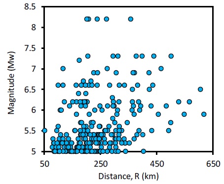
From the SSN database we selected 86 earthquakes (of various focal mechanism) located between 90.5° W and 96.5° W and between 13° and 17° N, and which occurred between 1995 and 2017. From this database, we present a wide range of magnitudes (5.0 ≤ Mw ≤ 8.2), distances (52 ≤ R ≤ 618 km; hipocentral distances for Mw<=7.0 and rupture distances for Mw> 7.0) and depths (10 ≤ H ≤ 243 km) as shown in Figure 1 and Table 1. We obtained 261 three-components accelerograms for those events recorded at 9 stations located in Chiapas, Oaxaca, Tabasco and Veracruz. The respective stations are OXJM, SCRU, NILT, MIHL, PIJI, TGBT, VHSA, SCCB and TAJN and belong to the Seismic Network of Institute of Engineering-UNAM (Pérez-Yáñez et al., 2010). Date, depth, moment magnitude (Mw) and distance for each recording are indicated in Table 1. The farthest away stations (VHSA and MIHL) have less recordings, in contrast with those sited in the central part of the study area (PIJI, NILT, SCCB, OXJM, TAJN, TGBT and SCRU) where the Chiapas State capital city (Tuxtla Gutierrez) and the hidroelectric dams are located.
Table 1 Earthquakes from southeastern Mexico analyzed in this study.
| No. | Date | Lat | Lon | H* | Mw | Distances of the records (km)* | No. | Date | Lat | Lon | H* | Mw | Distances of the records (km)* | ||||||||||||||||
| (dd/mm/yy) | (°N) | (°W) | (km) | MIHL | NILT | OXJM | PIJI | SCCB | SCRU | TAJN | TGBT | VHSA | (dd/mm/yy) | (°N) | (°W) | (km) | MIHL | NILT | OXJM | PIJI | SCCB | SCRU | TAJN | TGBT | VHSA | ||||
| 1 | 21/10/1995 | 16.92 | 93.64 | 165 | 7.2 | 92 | 47 | 13/03/2012 | 14.96 | -93.16 | 16 | 5.2 | 242 | 304 | 83 | 204 | 266 | 100 | 203 | 338 | |||||||||
| 2 | 03/06/2000 | 15.76 | -94.66 | 88 | 5 | 126 | 117 | 48 | 01/05/2012 | 14.11 | -93.16 | 40 | 6.1 | 181 | 298 | 140 | |||||||||||||
| 3 | 12/03/2000 | 14.59 | -92.97 | 35 | 5.9 | 165 | 308 | 49 | 26/06/2012 | 15.39 | -92.25 | 166 | 5.2 | 338 | 200 | 174 | |||||||||||||
| 4 | 17/10/2000 | 15.38 | -92.51 | 168 | 5.5 | 317 | 50 | 29/06/2012 | 14.78 | -93.3 | 18 | 5.3 | 303 | 103 | 228 | 117 | |||||||||||||
| 5 | 09/01/2001 | 15.36 | -93.24 | 66 | 6.1 | 248 | 51 | 12/07/2012 | 14.87 | -91.35 | 204 | 5.1 | 305 | ||||||||||||||||
| 6 | 19/01/2001 | 15.1 | -93.03 | 108 | 6.3 | 292 | 52 | 29/07/2012 | 14.1 | -92.82 | 14 | 5.7 | 183 | ||||||||||||||||
| 7 | 28/11/2001 | 15.41 | -93.64 | 36 | 6.4 | 172 | 198 | 53 | 01/09/2012 | 16.13 | -92.85 | 243 | 5.4 | 316 | 379 | 251 | 253 | ||||||||||||
| 8 | 16/01/2002 | 16.59 | -94.81 | 76 | 6.7 | 189 | 217 | 54 | 14/10/2012 | 14.46 | -92.73 | 13 | 5.2 | 148 | 251 | ||||||||||||||
| 9 | 14/02/2002 | 14.78 | -92.8 | 74 | 5.8 | 293 | 55 | 15/10/2012 | 13.77 | 13.77 | -91.48 | 20 | 288 | ||||||||||||||||
| 10 | 06/06/2006 | 15.37 | -91.86 | 209 | 5 | 260 | 220 | 56 | 27/10/2012 | 14.4 | -92.77 | 59 | 5 | 163 | |||||||||||||||
| 11 | 13/06/2007 | 13.26 | -91.43 | 20 | 6.6 | 336 | 208 | 57 | 07/11/2012 | 14.03 | -92.32 | 16 | 7.3 | 519 | 400 | 230 | 309 | 422 | 330 | 453 | |||||||||
| 12 | 06/07/2007 | 16.9 | -94.1 | 100 | 6.2 | 165 | 121 | 187 | 195 | 193 | 178 | 316 | 151 | 203 | 58 | 11/11/2012 | 14.06 | -92.48 | 13 | 6.2 | 199 | 296 | |||||||
| 13 | 23/07/2007 | 14.18 | -91.41 | 124 | 5.4 | 289 | 59 | 16/12/2012 | 14.43 | -91.66 | 100 | 5.4 | 244 | ||||||||||||||||
| 14 | 30/08/2007 | 15.68 | -93.9 | 61 | 5 | 141 | 98 | 192 | 60 | 30/12/2012 | 14.49 | -93.19 | 25 | 5.3 | 136 | ||||||||||||||
| 15 | 26/11/2007 | 15.28 | -93.36 | 87 | 5.6 | 218 | 280 | 100 | 199 | 245 | 190 | 317 | 61 | 31/12/2012 | 15.21 | -92.67 | 82 | 5.2 | 115 | ||||||||||
| 16 | 05/01/2008 | 13.83 | -92.12 | 63 | 5.6 | 248 | 62 | 11/01/2013 | 14.61 | -92.87 | 27 | 5.4 | 293 | 129 | 237 | ||||||||||||||
| 17 | 06/01/2008 | 13.99 | -92.03 | 20 | 5 | 231 | 63 | 11/01/2013 | 15.32 | -91.91 | 229 | 5 | 403 | 273 | |||||||||||||||
| 18 | 12/02/2008 | 16.19 | -94.54 | 90 | 6.6 | 220 | 100 | 182 | 238 | 117 | 196 | 282 | 64 | 25/03/2013 | 14.35 | -90.81 | 198 | 6.2 | 529 | 364 | 386 | 567 | |||||||
| 19 | 04/04/2008 | 13.85 | -91.59 | 73 | 5.1 | 282 | 65 | 10/05/2013 | 14.87 | -92.66 | 35 | 5.3 | 247 | ||||||||||||||||
| 20 | 15/04/2008 | 13.27 | -91.04 | 40 | 6.5 | 606 | 364 | 424 | 66 | 30/07/2013 | 15.5 | -93.33 | 105 | 5.4 | 214 | 108 | 189 | 246 | 246 | 246 | |||||||||
| 21 | 17/04/2008 | 15.45 | -93.52 | 95 | 5.4 | 198 | 259 | 196 | 226 | 182 | 67 | 06/08/2013 | 14.18 | -91.6 | 61 | 5.7 | 501 | ||||||||||||
| 22 | 20/09/2008 | 14.23 | -92.67 | 14 | 5 | 339 | 68 | 07/09/2013 | 14.34 | -92.26 | 69 | 6.1 | 484 | 367 | 431 | 196 | 276 | 394 | 295 | ||||||||||
| 23 | 16/10/2008 | 13.87 | -92.5 | 23 | 6.6 | 382 | 436 | 317 | 69 | 07/09/2013 | 14.14 | -92 | 51 | 5.4 | 401 | 225 | |||||||||||||
| 24 | 17/01/2009 | 15.74 | -92.76 | 171 | 5.2 | 284 | 353 | 178 | 203 | 326 | 210 | 70 | 10/01/2014 | 14.52 | 92.23 | 76 | 5 | 88 | |||||||||||
| 25 | 22/01/2009 | 15.19 | -91.93 | 199 | 5 | 251 | 71 | 11/01/2014 | 14.49 | -92.17 | 81 | 5.5 | 432 | 194 | 265 | 95 | |||||||||||||
| 26 | 03/05/2009 | 14.53 | -91.89 | 77 | 5.9 | 456 | 210 | 72 | 02/03/2014 | 14.08 | -93.26 | 10 | 5.7 | 180 | 301 | ||||||||||||||
| 27 | 07/06/2009 | 16.15 | -93.32 | 135 | 5 | 203 | 274 | 145 | 168 | 250 | 154 | 248 | 73 | 16/06/2014 | 15.1 | -91.89 | 14 | 5 | 161 | 197 | |||||||||
| 28 | 18/01/2010 | 13.85 | -90.67 | 124 | 5.9 | 548 | 618 | 370 | 74 | 07/07/2014 | 14.75 | -92.63 | 60 | 6.9 | 423 | 305 | 371 | 226 | 239 | 367 | |||||||||
| 29 | 23/02/2010 | 15.96 | -91.22 | 25 | 5.4 | 225 | 180 | 75 | 20/07/2014 | 14.76 | -92.58 | 80 | 5 | 313 | 231 | 89 | |||||||||||||
| 30 | 20/03/2010 | 16.03 | -91.32 | 50 | 5.3 | 219 | 171 | 76 | 29/07/2014 | 14.68 | -92.69 | 61 | 5.3 | 306 | 369 | 234 | 81 | 245 | |||||||||||
| 31 | 19/08/2010 | 14.41 | -91.84 | 40 | 5.2 | 212 | 85 | 77 | 28/08/2014 | 14.18 | -92.05 | 60 | 5 | 105 | |||||||||||||||
| 32 | 15/09/2010 | 15.59 | -93.52 | 95 | 5.1 | 189 | 253 | 102 | 186 | 170 | 78 | 15/10/2014 | 14.51 | -92.7 | 42 | 5.1 | 78 | ||||||||||||
| 33 | 01/11/2010 | 16.68 | -93.9 | 124 | 5 | 148 | 214 | 183 | 199 | 154 | 79 | 19/11/2014 | 14.71 | -93.39 | 25 | 5.2 | 240 | 129 | |||||||||||
| 34 | 20/01/2011 | 16.55 | -94 | 62 | 5.1 | 182 | 93 | 173 | 144 | 166 | 121 | 80 | 04/01/2015 | 16.29 | -94.27 | 99 | 5.1 | 213 | 173 | ||||||||||
| 35 | 27/03/2011 | 14.24 | -92.76 | 16 | 5.5 | 387 | 276 | 81 | 12/01/2015 | 15.39 | -93.41 | 82 | 5.5 | 326 | 205 | 268 | 190 | 160 | 178 | 305 | |||||||||
| 36 | 26/04/2011 | 15.88 | -92.74 | 138 | 5 | 149 | 82 | 20/01/2015 | 14.94 | -91.55 | 164 | 5.5 | 493 | ||||||||||||||||
| 37 | 07/06/2011 | 15.06 | -93.5 | 56 | 5.2 | 216 | 96 | 215 | 235 | 83 | 01/03/2015 | 13.37 | -91.01 | 40 | 5.3 | 226 | |||||||||||||
| 38 | 13/08/2011 | 14.58 | -94.88 | 16 | 5.7 | 224 | 218 | 224 | 346 | 84 | 01/05/2015 | 15.73 | 93.71 | 90 | 5 | 164 | 227 | 186 | 163 | ||||||||||
| 39 | 06/09/2011 | 16.25 | -93.82 | 93 | 5.1 | 133 | 205 | 131 | 170 | 137 | 85 | 15/05/2015 | 13.85 | -92 | 11 | 5.2 | 124 | ||||||||||||
| 40 | 19/10/2011 | 15.12 | -93.05 | 80 | 5 | 237 | 305 | 104 | 200 | 86 | 18/05/2015 | 14.07 | 92.13 | 62 | 5.2 | 114 | |||||||||||||
| 41 | 17/11/2011 | 14.52 | -92.42 | 20 | 5.5 | 158 | 52 | 87 | 01/09/2015 | 15.32 | -92.84 | 108 | 5.3 | 265 | 334 | 190 | 197 | 316 | |||||||||||
| 42 | 10/12/2011 | 15.33 | -94.79 | 16 | 5.2 | 140 | 88 | 17/12/2015 | 15.76 | -93.7 | 90 | 6.6 | 163 | ||||||||||||||||
| 43 | 20/12/2011 | 13.81 | -93.43 | 15 | 5.1 | 211 | 89 | 14/06/2017 | 14.77 | -92.08 | 113 | 7 | 465 | 116 | 274 | ||||||||||||||
| 44 | 21/01/2012 | 14.74 | -93.24 | 16 | 6 | 390 | 255 | 311 | 107 | 230 | 111 | 363 | 90 | 07/09/2017 | 14.85 | -94.11 | 58 | 8.2 | 273 | 121 | 112 | 272 | 77 | ||||||
| 45 | 16/02/2012 | 14.59 | -92.92 | 25 | 5 | 291 | 129 | 239 | 85 | Total records | 10 | 44 | 30 | 57 | 43 | 20 | 24 | 22 | 11 | ||||||||||
| 46 | 20/02/2012 | 14.37 | -93.14 | 16 | 5.2 | 148 | 116 | ||||||||||||||||||||||
* H represents focal depth.
The spatial distribution of the 9 accelerometric stations (red squares), and of the 86 epicenters (white and black circles) is shown in Figure 1. Also indicated are the locations of the Chiapas (AVC) and Guatemala (AVCA) volcanic arcs. The Chiapas Massif is depicted in pink. Figure 1 also shows the Polochic-Motagua (continuous red line), Tonalá and Los Tuxtlas (discontinuous red line) fault systems. The epicenter of the Tehuantepec, September 7, 2017 (Mw8.2) earthquake is indicated with a green star. Green small dots represent aftershocks with magnitudes lower than 5. A comparison of the area covered by the aftershocks of the Tehuantepec earthquake with the localized seismicity of the last 17 years indicates that the Tehuantepec aftershocks cover that portion of the Tehuantepec Gulf that had been inactive.
In the right panel of Figure 1. The 261 hypocenters analyzed in this study were projected to the A-A´ cross-section (right panel of Figure 1), whose location is indicated with a white line. A dipping angle of the slab of about 45 degrees, as well as a plate thinning at 80 km depth can be observed.
Stars indicate the epicenters of the three earthquakes with Mw > 7.0 (see Table 1). For these events, the minimum distance to the rupture was considered. For the October 21, 1995 earthquake (Mw 7.2), according to the rupture model proposed by Rebollar et al. (1999), the rupture depth (htop) lies at 80 km. For the September 8, 2017 event (Mw 8.2), we used the rupture model obtained by Ye et al. (2017), which has a htop = 30 km. Finally, for the November 7, 2012 (Mw 7.3) event, for which there is no rupture model, we assumed a rupture model with a htop = 10 km, with its closest edge point (northwestern edge of the fault plane) at latitude 14º N and longitude 92º W.
Figure 2 shows the distribution of magnitudes (5.0 ≤ Mw ≤ 8.2) versus distance (52 ≤ R ≤ 618 km) of the analyzed records. A concentration of events with magnitudes in the range from 5.0 to 5.5 for distances between 52 and 300 km is observed.
Data Processing and Analysis
For each of the three components of the 261 recordings associated to the 86 selected seismic events, both shear waves and surface waves (also known as coda) were selected. Data processing included homogenization of the signal sampling of all extracted signals. Subsequently, for each selected record, the Fourier amplitude spectrum (FAS) was computed and the spectral ratio of horizontal components with respect to the vertical one obtained. After that, the quadratic means were obtained from both ratios. These are the directional earthquake horizontal to vertical spectral ratios (EHVSR), which were computed for a frequency band between 0.1 and 10 Hz. In Figure 3 we show the 261 ratios (thin of colors continuous lines) distributed in the 9 stations. Averages are depicted as continuous red lines (dashed red lines: average ± one standard deviation). We assume that this average of directional EHVSR´s is an estimate of the spectral amplification, a kind of empirical transfer function (ETF) of average horizontal components with respect to the vertical component. The source effect is approximately removed. In a recent paper, Kawase et al. (2018) suggested to consider the amplification due to vertical motion to avoid over-reduction of FAS. However, this requires recordings both in soil and rock sites.

Figure 3 Earthquake horizontal to vertical spectral ratios EHVSR at the nine studied stations. In thin of colours continuous lines, the quadratic mean spectral ratios (continuous red lines) of each earthquake are plotted in log-log scale (dashed red lines: average ± one standard deviation). The trends are clear and the averages at each station, depicted in red, are assumed to represent the site effect. The value of two suggested by SESAME (2000), continuous line, and the theoretical H/V in a Poissonian half-space are given as reference (discontinuous line).
It has been proposed that the site effect is significant for ETF larger than two (SESAME, 2015) as it is the case of scalar amplification in a half-space. However, under the assumption of a diffuse field, Sánchez-Sesma et al. (2011a) found theoretically that the MHVSR at the surface of a half-space is approximately given by
where v=Poisson ratio. If v =0.25 then the H/V is about 1.332.
Thus, according to criteria from SESAME (continuous line in Figure 3), and to that of Sánchez-Sesma et al. (2011) (discontinuous line in Figure 3), the 9 accelerometric stations present site effects in the analyzed frequency band. Stations NILT and PIJI reach amplifications of more than ten times at 6 and 4 Hz, respectively. Stations OXJM, SCRU and TGBT present lower amplifications.
Finally, to suppress site effects from the 261 records, with the ETF computed previously (red continuous line, Figure 3) and the estimated FAS for each record, we compute the deconvolution between the FAS for the nine sites and ETF in the frequency domain for this site, subtracting their respective site effect. The corresponding intensities (spectral acceleration and peak values) are estimated using random vibration theory (RVT) (i.e., Arciniega-Ceballos 1990; Reinoso and Ordaz 1999), which comprises the following steps: (1) de-amplifying the FAS by dividing them by the EHVSR obtaining a proxy of ETF; (2) multiplication of the spectrum by the oscillator transfer function or by one if PGA is seek; (3) calculation of the moments m
0
and m
2
of the power density which are given by
In this way, the estimated ground motion intensities (e.g. acceleration response spectra) for each event and site will be essentially free of site effect. In Figure 4 this reduction is illustrated for the July 6th, 2007 (Mw=6.2) event. The complex Fourier spectra were deconvolved by the corresponding average EHVSR (ETF) and then transformed back to time domain. The N-S accelerograms of the nine stations are displayed in the left panel. The corresponding distance and PGA are indicated. In the right panel the recordings with suppressed site effect are displayed (as if the corresponding stations were located in hard rock). This suppression gives significantly lower PGA values (for TAJN a factor of 7.5 was obtained). We claim that the use of average EHVSR may be adequate to correct GMPE for site effects, leading to a more realistic attenuation model.
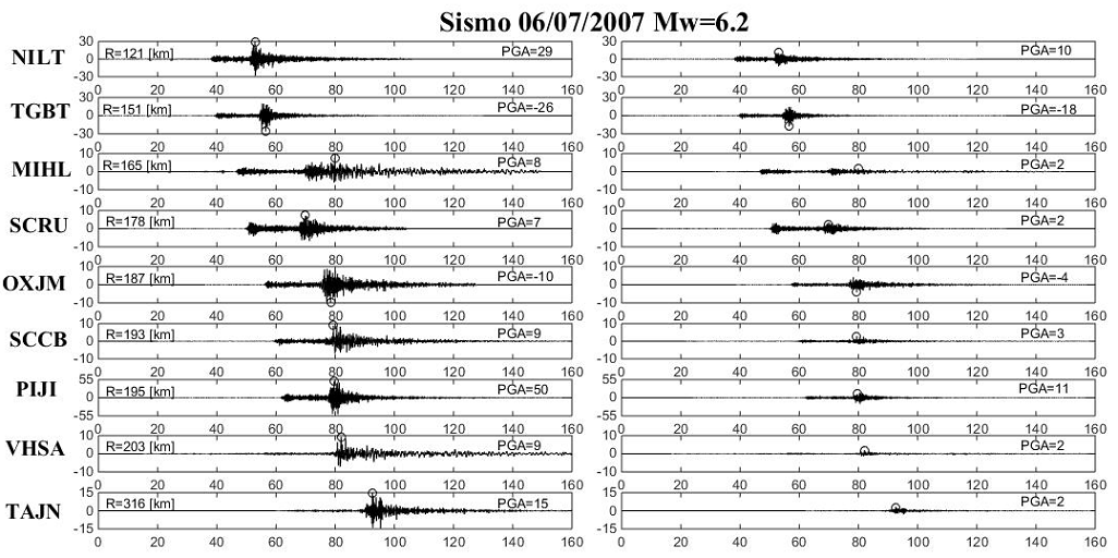
Figure 4 Example of site effects correction for a Mw=6.2 event of July 6th , 2007 for the studied stations. Left panel depicts the N-S accelerations indicating the epicentral distance and the PGA in gals (cm/s2). The right panel shows the time series with the site effects removed with the procedure described herein.
Peak ground accelerations (PGA) are obtained from these corrected records. Also, response spectra with 5 % critical damping are obtained for 24 structural periods ranging between 0.3 and 40 Hz. Finally, peak ground velocities are obtained by integrating these recordings after correcting them for base line (Boore, 2005) and band-pass filtering between 0.3 and 40 Hz.
Each parameter (i.e., PGA, PGV, or the spectral ordinates) is separately calculated for both horizontal components, then the quadratic mean is obtained from both ortogonal components (Boore, 2005). Other alternatives would include the geometric mean, or other no geometrical means (Boore, 2010). We used the quadratic vector mean as it is a common practice in the development of attenuation models, since from the physics point of view it is more rational than other means. All recordings were processed in the same form.
Regression analysis
To estimate the spectral accelerations with a damping of 5 %, as well as the PGA and PGV, the regression analysis of the data set was made using the maximal verisimilitude method of one stage proposed by Boore (1993), which constitutes the most direct form to predict the response spectra of observed data. We use a simpler functional form proposed by Ordaz et al. (1989), and García-Soto and Jaimes (2017) to estimate the spectral ordinates, PGA, and PGV for seismic events from southeastern Mexico.
where Y(T) represents the horizontal spectral ordinate based on a quadratic mean of the horizontal components, T in seconds is the period of the single degree of freedom system, Mw is the moment magnitude, R is the closest distance from site to fault surface for larger events (Mw > 6.5) or the hypocentral distance for the rest, both in km, i are the coefficients estimated by the regression analysis, and ε1 is the error estimation by assuming a normal distribution.
Noteworthy is that in previous studies (i.e., Arroyo, 2010; García-Soto and Jaimes, 2017) no important dependence with the focal depth was found, consequently it was not considered in excluded from this study. Even more, the quadratic mean was used since the use of the geometric mean and was the development of the attenuation relationship is slightly less conservative than the use of the quadratic mean to evaluate seismic risk (i.e., Hong and Goda, 2007). The horizontal geometric dispersion can be obtained as G(R)=Rα 3 (T), where α3(T) is the geometric attenuation coefficient, which controls the amplitude decay with the distance, R. By applying the natural logarithm to both sides of the last expression, it can be linearized as ln(G(R))=α3(T)∙lnR, which corresponds to the third term of equation (2). In this study, it was considered that α3(T) is very well constrained by seismic observations in intraplate events (i.e., Ordaz et al. 1994; Reyes, 1999; Jaimes et al. 2006; Garcia-Soto and Jaimes, 2017). Further, by fixing the geometric dispersion coefficient at -0.5 for all the ordinates in both components (i.e., Ordaz et al., 1994; Reyes, 1999; Jaimes et al., 2006), unrealistic values are avoided (i.e., non-negative values of α3(T),) that physically have no sense (Ordaz et al. 1994).
Results and Discussion
Regression Coefficients and Residuals
Regression coefficients, αi(T), and the standard deviation σi(T), were estimated for periods T between 0.1 and 10 s, for recordings of 4 groups: Group 1, considers all recordings without site effects; Group 2, includes the recordings with site effects; Group 3, comprises recordings of earthquakes with depths less than 80 km but without site effects; while Group 4, is constituted by recordings of earthquakes with depths less than 250 km and no corrected for site effects. Figure 5 shows, in a logarithmic scale, the values of the regression coefficients α1(T), α2(T) and α4(T) for period values between 0.1 and 10 s. No differences significant are found between coefficients α2 and α4 among the 4 groups. However, coefficient α1 of group 2 (which includes site effects) shows an evident divergence, from the others groups. Confirmation of the validity of the attenuation model is indicated by the standard deviation σi(T) obtained for the cases with and without site effects. Table 2 summarizes the regression coefficients αi(T) and the standard deviation obtained from the analyzed recordings by considering the quadratic mean of the horizontal components.
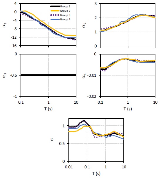
Figure 5 - Regression coefficients and natural logarithmic standard deviation logarithmic for horizontal components in the sites of Chiapas State, Mexico. a) Group 1: all records without site effects. B) Group 2 all records presenting site effects, c) Group 3 including records with depths less than 80 km, and d) Group 4 with records with depths less than 250 km and no site effect.
Table 2 Regression coefficients obtained for the horizontal components.
| Grupo 1 | Grupo 2 | |||||||
| T (s) | α1 | α2 | α4 | α | α1 | α2 | α4 | α |
| 0.01 | -1.5508 | 1.1515 | -0.0066 | 0.96 | -1.1789 | 1.2033 | -0.0057 | 0.84 |
| 0.02 | -1.5518 | 1.1516 | -0.0066 | 0.96 | -1.1802 | 1.2036 | -0.0057 | 0.84 |
| 0.04 | -0.9102 | 1.1402 | -0.0070 | 1.08 | -0.8432 | 1.2014 | -0.0062 | 0.90 |
| 0.06 | 0.0273 | 1.0727 | -0.0077 | 1.13 | -0.2829 | 1.1604 | -0.0067 | 0.97 |
| 0.08 | 0.1705 | 1.0758 | -0.0074 | 1.12 | 0.0004 | 1.1415 | -0.0067 | 0.99 |
| 0.1 | -0.0772 | 1.0803 | -0.0071 | 1.06 | 0.2687 | 1.1119 | -0.0065 | 0.98 |
| 0.2 | -1.8836 | 1.2276 | -0.0060 | 0.84 | -0.3723 | 1.2176 | -0.0060 | 0.85 |
| 0.3 | -3.3412 | 1.3582 | -0.0043 | 0.75 | -1.5325 | 1.3277 | -0.0048 | 0.78 |
| 0.4 | -4.1157 | 1.4207 | -0.0036 | 0.74 | -2.8650 | 1.4583 | -0.0039 | 0.72 |
| 0.5 | -5.0784 | 1.5269 | -0.0029 | 0.74 | -3.9424 | 1.5641 | -0.0031 | 0.72 |
| 0.6 | -5.7386 | 1.5918 | -0.0025 | 0.74 | -4.5830 | 1.6097 | -0.0025 | 0.74 |
| 0.7 | -6.1632 | 1.6285 | -0.0025 | 0.71 | -5.0980 | 1.6559 | -0.0025 | 0.72 |
| 0.8 | -6.7363 | 1.6862 | -0.0023 | 0.73 | -5.6886 | 1.7072 | -0.0022 | 0.73 |
| 0.9 | -7.2001 | 1.7347 | -0.0023 | 0.74 | -6.1589 | 1.7580 | -0.0022 | 0.74 |
| 1 | -7.5814 | 1.7794 | -0.0024 | 0.74 | -6.6258 | 1.8121 | -0.0023 | 0.76 |
| 1.1 | -7.9202 | 1.8218 | -0.0026 | 0.72 | -6.9805 | 1.8454 | -0.0024 | 0.74 |
| 1.2 | -8.2500 | 1.8662 | -0.0029 | 0.72 | -7.2676 | 1.8767 | -0.0026 | 0.74 |
| 1.3 | -8.6025 | 1.9053 | -0.0029 | 0.74 | -7.5384 | 1.9029 | -0.0027 | 0.76 |
| 1.4 | -8.9040 | 1.9359 | -0.0029 | 0.75 | -7.8037 | 1.9253 | -0.0026 | 0.77 |
| 1.5 | -9.1855 | 1.9686 | -0.0030 | 0.75 | -8.0682 | 1.9535 | -0.0026 | 0.77 |
| 1.6 | -9.3861 | 1.9875 | -0.0031 | 0.74 | -8.2767 | 1.9731 | -0.0027 | 0.77 |
| 1.7 | -9.6182 | 2.0066 | -0.0030 | 0.73 | -8.5064 | 1.9932 | -0.0027 | 0.77 |
| 1.8 | -9.8511 | 2.0287 | -0.0030 | 0.73 | -8.7205 | 2.0161 | -0.0028 | 0.78 |
| 1.9 | -10.0840 | 2.0525 | -0.0031 | 0.74 | -8.8946 | 2.0317 | -0.0028 | 0.79 |
| 2 | -10.3230 | 2.0783 | -0.0030 | 0.75 | -9.0643 | 2.0470 | -0.0029 | 0.80 |
| 2.1 | -10.5020 | 2.1001 | -0.0031 | 0.76 | -9.2065 | 2.0651 | -0.0031 | 0.81 |
| 2.2 | -10.6030 | 2.1060 | -0.0032 | 0.77 | -9.3423 | 2.0806 | -0.0032 | 0.81 |
| 2.3 | -10.6940 | 2.1132 | -0.0033 | 0.77 | -9.4559 | 2.0931 | -0.0033 | 0.82 |
| 2.4 | -10.8300 | 2.1258 | -0.0033 | 0.78 | -9.5928 | 2.1075 | -0.0033 | 0.82 |
| 2.5 | -10.9520 | 2.1373 | -0.0033 | 0.78 | -9.7241 | 2.1211 | -0.0034 | 0.83 |
| 2.6 | -11.0450 | 2.1454 | -0.0034 | 0.78 | -9.8505 | 2.1347 | -0.0035 | 0.83 |
| 2.7 | -11.1190 | 2.1487 | -0.0035 | 0.78 | -9.9396 | 2.1407 | -0.0035 | 0.83 |
| 2.8 | -11.2020 | 2.1547 | -0.0036 | 0.78 | -10.0500 | 2.1501 | -0.0036 | 0.83 |
| 2.9 | -11.2640 | 2.1582 | -0.0036 | 0.78 | -10.1420 | 2.1582 | -0.0036 | 0.84 |
| 3 | -11.3170 | 2.1597 | -0.0037 | 0.78 | -10.2080 | 2.1620 | -0.0037 | 0.84 |
| 4 | -12.0000 | 2.1999 | -0.0036 | 0.76 | -11.0170 | 2.2074 | -0.0034 | 0.80 |
| 10 | -12.9230 | 2.1268 | -0.0037 | 0.71 | -11.2190 | 2.0019 | -0.0031 | 0.68 |
| PGA | -1.5528 | 1.1517 | -0.0066 | 0.96 | -1.1804 | 1.2035 | -0.0057 | 0.84 |
| PGV | -7.9782 | 1.5989 | -0.0045 | 0.69 | -5.2675 | 1.3045 | -0.0015 | 0.72 |
| Grupo 3 | Grupo 4 | |||||||
| T (s) | α1 | α2 | α4 | α | α1 | α2 | α4 | α |
| 0.01 | -2.4021 | 1.2740 | -0.0068 | 0.94 | -0.6243 | 1.0278 | -0.0066 | 0.92 |
| 0.02 | -2.4032 | 1.2741 | -0.0068 | 0.94 | -0.6255 | 1.0280 | -0.0066 | 0.92 |
| 0.04 | -1.9104 | 1.2753 | -0.0070 | 1.07 | 0.2756 | 0.9883 | -0.0072 | 1.00 |
| 0.06 | -0.9018 | 1.2115 | -0.0081 | 1.14 | 0.8888 | 0.9587 | -0.0074 | 1.03 |
| 0.08 | -0.7548 | 1.2182 | -0.0079 | 1.12 | 1.0427 | 0.9535 | -0.0071 | 1.04 |
| 0.1 | -0.8250 | 1.1929 | -0.0075 | 1.05 | 0.4859 | 1.0117 | -0.0068 | 0.99 |
| 0.2 | -2.4394 | 1.3187 | -0.0066 | 0.77 | -1.6079 | 1.1957 | -0.0055 | 0.86 |
| 0.3 | -3.7200 | 1.4183 | -0.0047 | 0.67 | -3.2780 | 1.3628 | -0.0039 | 0.79 |
| 0.4 | -4.3712 | 1.4573 | -0.0038 | 0.68 | -4.1248 | 1.4403 | -0.0034 | 0.77 |
| 0.5 | -5.0664 | 1.5030 | -0.0027 | 0.70 | -5.5705 | 1.6473 | -0.0030 | 0.75 |
| 0.6 | -5.6933 | 1.5746 | -0.0027 | 0.69 | -6.4074 | 1.7271 | -0.0023 | 0.75 |
| 0.7 | -6.1841 | 1.6204 | -0.0026 | 0.70 | -6.6099 | 1.7249 | -0.0024 | 0.71 |
| 0.8 | -6.7908 | 1.6798 | -0.0023 | 0.73 | -7.0916 | 1.7708 | -0.0023 | 0.71 |
| 0.9 | -7.2440 | 1.7291 | -0.0022 | 0.75 | -7.4292 | 1.7927 | -0.0023 | 0.70 |
| 1 | -7.4932 | 1.7537 | -0.0024 | 0.77 | -8.1831 | 1.8992 | -0.0023 | 0.68 |
| 1.1 | -7.8381 | 1.7911 | -0.0025 | 0.76 | -8.5043 | 1.9452 | -0.0026 | 0.66 |
| 1.2 | -8.2195 | 1.8408 | -0.0027 | 0.74 | -8.7325 | 1.9763 | -0.0030 | 0.67 |
| 1.3 | -8.5256 | 1.8707 | -0.0028 | 0.76 | -9.1991 | 2.0367 | -0.0031 | 0.69 |
| 1.4 | -8.7945 | 1.8908 | -0.0027 | 0.77 | -9.6278 | 2.0958 | -0.0031 | 0.71 |
| 1.5 | -9.0462 | 1.9132 | -0.0027 | 0.77 | -9.9370 | 2.1393 | -0.0034 | 0.71 |
| 1.6 | -9.2658 | 1.9325 | -0.0028 | 0.74 | -10.1650 | 2.1670 | -0.0035 | 0.71 |
| 1.7 | -9.5299 | 1.9576 | -0.0027 | 0.73 | -10.3090 | 2.1700 | -0.0034 | 0.70 |
| 1.8 | -9.7789 | 1.9782 | -0.0026 | 0.74 | -10.4910 | 2.1886 | -0.0035 | 0.69 |
| 1.9 | -10.0690 | 2.0087 | -0.0026 | 0.75 | -10.6570 | 2.2050 | -0.0036 | 0.70 |
| 2 | -10.3500 | 2.0384 | -0.0025 | 0.76 | -10.7930 | 2.2171 | -0.0036 | 0.72 |
| 2.1 | -10.5730 | 2.0661 | -0.0026 | 0.77 | -10.8310 | 2.2162 | -0.0038 | 0.72 |
| 2.2 | -10.6890 | 2.0764 | -0.0026 | 0.77 | -10.8720 | 2.2093 | -0.0038 | 0.73 |
| 2.3 | -10.8370 | 2.0959 | -0.0028 | 0.78 | -10.8630 | 2.1960 | -0.0039 | 0.73 |
| 2.4 | -11.0080 | 2.1167 | -0.0029 | 0.79 | -10.9130 | 2.1914 | -0.0038 | 0.73 |
| 2.5 | -11.1280 | 2.1300 | -0.0029 | 0.80 | -11.0370 | 2.2001 | -0.0038 | 0.73 |
| 2.6 | -11.2220 | 2.1403 | -0.0031 | 0.80 | -11.1400 | 2.2076 | -0.0038 | 0.73 |
| 2.7 | -11.3120 | 2.1481 | -0.0032 | 0.80 | -11.1990 | 2.2063 | -0.0038 | 0.73 |
| 2.8 | -11.3780 | 2.1511 | -0.0032 | 0.80 | -11.3060 | 2.2163 | -0.0039 | 0.72 |
| 2.9 | -11.4150 | 2.1518 | -0.0033 | 0.81 | -11.3910 | 2.2223 | -0.0040 | 0.73 |
| 3 | -11.4340 | 2.1479 | -0.0034 | 0.82 | -11.4980 | 2.2325 | -0.0040 | 0.72 |
| 4 | -12.0980 | 2.1843 | -0.0032 | 0.80 | -12.0520 | 2.2499 | -0.0041 | 0.70 |
| 10 | -13.1860 | 2.1597 | -0.0034 | 0.77 | -12.1180 | 2.0009 | -0.0041 | 0.62 |
| PGA | -2.4043 | 1.2743 | -0.0068 | 0.94 | -0.6286 | 1.0285 | -0.0066 | 0.92 |
| PGV | -8.4826 | 1.6581 | -0.0045 | 0.68 | -7.5498 | 1.5644 | -0.0047 | 0.65 |
*Coefficient α3 was fixed at -0.50 for the horizontal components.
**Coefficient α3 was fixed at -0.50 for the horizontal components.
For the purpose of this analysis, the residual is defined as:
where ln(Yi) is the natural logarithm of i-eth observed value Y
i and

Figure 6 Residual values obtained from the regression of the horizontal components according to magnitude (upper part of panel), and with respect to distance (lower part of each panel) for peak ground acceleration (PGA) and spectral pseudoaceleration, Sa, at T values of 0.06, 0.5, and 1 s. Panel a comprises all records without site effect, panel b includes all records with site effect, panel c considers records with depths less than 80 km and without site effect. Finally, panel d corresponds to records with depth less than 250 without site effect.
Comparison with Other Studies
To the author's knowledge, there are no GMPEs in the region under study, which makes the outcome more necessary to compute the seismic hazard in the region. For that reason, the Figure 7 compares the attenuation model obtained in this study (for magnitudes Mw of 5.5, 6.5, and 7.5) with those of García et al., (2005), Arroyo et al., (2010) and García-Soto and Jaimes (2017), based on earthquakes located at the Pacific Ocean coasts (discontinuous lines). Attenuation models obtained in this study present a slower decay than previous ones, and models that include site effects (yellow lines) present larger amplitudes than those without site effects (black lines). Previous attenuation models are clearly different to the attenuation models here presented for southeastern Mexico. These differences could be due to the fact that in southeastern Mexico earthquakes attain depths up to about 243 km, while in the Guerrero coast (southern Mexico) depths are less than 80 km. In general, models by Arroyo et al. (2010) and Garcia-Soto and Jaimes (2017) follow a similar pattern in all cases, and for Sa, for T = 0.5 s and 1 s, they decay almost in the same way as the model by Garcia (2005) for Mw 5.5 and 6.5. For PGA, the model by Garcia (2005) present larger amplitudes (for the three magnitudes) than those by the models by Arroyo et al. (2010) and Garcia-Soto and Jaimes (2017). In particular, the PGA models corrected for site effects (obtained in this study) have smaller amplitudes than the models by Arroyo et al. (2010) and Garcia-Soto and Jaimes (2017) only for distances smaller than 130, 90 and 50 km for Mw 5.5, 6.5 and 7.5, respectively. On the contrary, Sa models corrected for site effects present lower amplitudes than those of the previous models. However, and as it was expected, the corresponding models that include site effects (yellow lines) present the largest amplitudes at all distances. In other words, a model comprising site effects presents overestimated values.
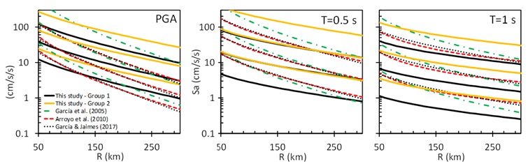
Figure 7 Regression curves for the horizontal component for PGA and spectral pseudo-acceleration, Sa, for periods of 0.5 and 1 s for earthquakes with magnitudes Mw of 5.5, 6.5, and 7.5. Group 1 comprises regression of all records without site effect, while group 2 includes all records with site effect.
CONCLUSIONS
We present an attenuation model for strong motion for southeastern Mexico which is approximately free of local amplification. This means that the GMPE thus obtained can be regarded as appropriate for firm ground. This was accomplished using average EHVSR to construct an empirical transfer function (ETF) for each site to perform a spectral deconvolution on observed records. A statistical regression model was adjusted to construct the corrected GMPE. The model is built as a function of the magnitude and distance from 86 seismic events with magnitudes 5.0 ≤ Mw ≤ 8.2, and distances 52 ≤ R ≤ 618 km recorded at the states of Chiapas, Oaxaca, Tabasco and Veracruz.
This study shows a practical, approximate approach to remove the site effect in the ground motion attenuation models, the so called GMPE. Otherwise, the seismic intensities could be overestimated. Such is the case in the current values of regulatory norms for the study region. We approximately suppress site effects at the accelerometric stations which provide data to construct attenuation models using the average EHVSR. The aim is to obtain reasonable seismic intensities without the bias induced by local site effects.

