


 nueva página del texto (beta)
 Inglés (pdf)
 Artículo en XML
 Referencias del artículo
 Enviar artículo por email
 Citado por SciELO
  Similares en
SciELO
Similares en
SciELO 
 Permalink
Introduction
Geostrophic balanced flows for large scale, steady, mean flow are the primordial ingredient to decipher and understand long term effects of the ocean circulation (e.g., Wunsch and Ferrari, 2019). The thermal wind equation (e.g., system (7) in Wunsch and Ferrari, 2019) is the classical step to infer absolute geostrophic velocities at depth. However, it needs reference velocities or directional constraints that vary with depth. The classical study of Stommel and Schott (1977), or, for example, Needler (1985) and Chu (1995), address the topic of achieving the geostrophic reference velocity from directional constraints. These studies are done using potential isopycnal surfaces as material surfaces, which is the common shortcut to deal with compressibility. In the incompressible fluid limit, the intersection of isopycnal and iso-potential vorticity surfaces set the direction of geostrophic flows. In this study, the ocean fluid compressibility is amply considered, without the need of global material surfaces.
Present-day knowledge of the mean surface circulation (e.g., Niiler et al., 2003; Chu, 2020) provides, directly, the integration constant, although for abyssal flows such reference velocity is far away; hence the integration is prone to cumulative errors for the deep, slow motion environment. Deep flows still deserve the traditional perspective: Do mean hydrographic distributions allow a robust estimate, via geostrophic and other approximate balances, of the mean circulation? The question of determining flow properties with hydrographic information alone still deserves attention. The essential physical nature of conditions to derive the absolute (mean) velocity are given in numerous studies, all of which relate to thermocline theories, for example Behringer (1979), Chu (1995), Coats (1981), Davis (1978), Killworth (1984), Killworth (1986), Needler (1985), Olbers and Willebrand (1984), Stommel and Schott (1977), McDougall (2013) and Wunsch (1994), to mention just a few. This list is far from exhaustive, but all of them deal with mapping potential vorticity on some sort of isopycnal surfaces. Any simplified thermodynamic and dynamical models in use have corresponding reduced versions of the mass and potential vorticity conservations, and therefore directional constraints.
Jackett and McDougall (1997) argue that for the compressible ocean fluid, a better approximation than potential density iso-surfaces are the ‘Neutral surfaces’, in which case the intersection of ‘Neutral surfaces’ and iso-potential vorticity surfaces set the directional constraints. Alternatives to ‘Neutral surfaces’ are the ‘Orthobaric surfaces’ (de Szoeke et al., 2000), ‘Topobaric surfaces’ (Stanley, 2019), as proposed by Eden and Willebrand (1999) or Klocker et al. (2009), all these versions are here considered as improvements of potential isopycnals. Examples of flow trajectories, under several simplifying assumptions, are commonly shown by plotting contours of potential vorticity over these improvements of potential isopycnals (Needler, 1985; McDougall, 2013; Chu, 2000). This practice is used even in numerical models (Zhang et al., 2003). Before the advent of ‘Neutral surfaces’, or its close relatives (i.e., ‘Orthobaric’, ‘Topobaric’ and others), iso-potential densities surfaces were used with the same purpose (Coats, 1981).
Even in numerical studies, trajectories to characterize flow properties are useful, for example, in Malanotte-Rizzoli et al. (2000), following Killworth (1986), contours of the Bernoulli function along outcropping isopycnal surfaces signal distinctive features of the North Atlantic Subtropical Cell. These trajectories are in agreement with observations shown by Zhang et al. (2003), which benefit from direct measurements of the surface circulation and therefore allows the determination of the Bernoulli function.
In addition to the polemic concept of ‘Neutral surfaces’ (Tailleux, 2016, McDougall et al., 2017, Tailleux, 2017), Bennett (2019) points out the ill-defined mathematical problem of constructing ‘Neutral surfaces’, which is a well-known limitation (McDougall and Jackett, 1988, McDougall, 1995). We show here that ‘Neutral surfaces’ are unnecessary for determining flow trajectories. This study shows that, without the incompressibility and Boussinesq approximations, the fundamental restrictions (i.e., orthogonality conditions on the velocity field) that oblige the conservation of ‘local’ potential density, and potential vorticity in their limit of the geostrophic steady mean flow, fully define unique trajectories; here called ‘Preferred Trajectories’. The added condition, brought by the conservation of potential vorticity, on the neutral trajectories of Bennett (2019) selects a unique subset of them (i.e., the ‘Preferred Trajectories’).
The following section presents the theory, framed within some historical perspective, as well as the discussion, a third section shows examples of ‘Preferred Trajectories’ in the North Atlantic, and the fourth and last section summarizes the conclusion.
Theory and discussion
A) Background theory
Under steady, adiabatic, non-diffusive, geostrophic, and incompressible flow conditions, the equations
and
Where ρ and u are the mass density and velocity fields respectively, z is the vertical coordinate in the direction opposite to gravity, and f = 2Ωsinφ is the Coriolis parameter (Ω is the magnitude of Earth’s angular velocity, φ is the latitude), are the conservations of mass and potential vorticity. It should be noted that the incompressibility approximation is far from valid in deep regions, but required for system (1). These constraints on velocity, or their close relatives in less simplified models, are the prime candidates for determining ‘absolute’ geostrophic velocities. The reason for naming ‘absolute’ the velocities derived under such constraints is that provided the isopycnal and iso-potential vorticity surfaces do not coincide, they determine the, previously free, integration constants of the thermal wind equations.
Compressibility effects make Eq (1.1) useless when dealing with the global-scale flow, but modified versions of system (1) might be acceptable. A thermodynamic variable not affected by compressibility is salinity (S), hence the equation
implies that displacements take place along isohaline surfaces (i.e., isohaline surfaces are then material surfaces), and therefore is another candidate to help determine constants in the integration of the thermal wind equations. However, for this equation to hold, non-diffusive conditions are the natural requisite. A similar non-diffusive condition on heat does not imply displacements along isotherms (neither on constant potential temperature surfaces, except for the pressure level where the potential temperature is referenced to). Under non-diffusive and adiabatic conditions, and allowing for compressibility, the temperature equation reads:
where T is temperature, P is pressure and Γ = Γ (P,T ,S ) is the adiabatic temperature lapse rate (i.e., Γ = (δT / δP) s,η , the partial derivative of temperature respect to pressure at constant salinity and entropy (η)). Rewriting ( Eq. 2.2) as u (∇T - Γ∇P) = 0, serves better to show the orthogonality condition explicitly.
Let us remind first that, system (2) under large-scale zero-order dynamics might provide the constraint on the direction. Only in regions where ∇S and ∇T - Γ∇P are neither null nor parallel (i.e., linearly independent) system (2) restricts u to be unidirectional.
At this point, it should be mentioned the need for the equations of state
to deal with compressibility issues (i.e., sound speed).
Below we show that other orthogonality conditions, besides system (2), arise closer to dynamical balances.
The reduction of the equations of motion to a geostrophic and hydrostatic balance, proper for large-scale motions, is stated by:
where λ is the longitude, φ is the latitude, r is the radial (or vertical z ) coordinate, u and v are the zonal and meridional velocity components and g is the magnitude of gravity. ( Eq.s 4.1) to (4.3) can be rewritten as ∇P = ρfve λ - ρfue φ - ρge r where e λ , e φ and e r are the unitary vectors in the zonal, meridional and radial (vertical) directions; a spherical coordinate system where u = ue λ + ve φ + we r with w as the vertical component of velocity and g = - ge r . Mass conservation is expressed by
Notice the absence of the incompressibility and Boussinesq approximations in system (4). The mass flux density (i.e., ρu ) is used throughout the rest without needing a Boussinesq approximation. The null rotational of ∇P defines the thermal wind equations and, in addition with Eq. (4.4), the Svedrup relationship or vorticity equation, in the geostrophic approximation:
where β= r -1 df / dφ = r -1 2Ωcosφ . The horizontal divergence of the mass density flux (i.e., of ρu ) allowed in the large-scale geostrophic balance relates (via ( Eq. 4.4), the mass conservation) the ‘vertical’ stretching/contraction of seawater parcels with their meridional excursion; ( Eq.5.3) is the Svedrup relation. Notice that geometric factors, pertinent to the spherical frame of reference, modify the usual ‘Cartesian’ expressions of the conventional β -plane approximation (i.e., ( Eq.5.3) reduces to βv = f𝜕w / 𝜕z under the notation and approximations assumed in system (1). From system (4) it follows that
This result is slightly more general, because ( Eq.s 4.1) to (4.3) are 2ρ𝝕× u = -∇P + ρ g , where 𝝕 is Earth’s angular velocity, with the horizontal component of 𝝕 neglected. Notice in the previous notation (i.e., f =2Ωsinφ in ( Eq.1.2)), Ω is |𝝕 |. This slightly more general Eq. than Eq.s (4.1) to (4.3), also leads, in the simple incompressible limit (see Killworth, 1986), to the conservation of the Bernoulli function (i.e., u ‧ ∇(P + gρz) = 0 , where P + gρz is the Bernoulli function).
B) Material surfaces and inexact differentials.
For any differentiable vector field C = C ( r ) where r is the position vector, a valid temptation is to build surfaces (or contours in 2D) such that a scalar function γ = γ ( r ) solves the differential form dγ = C ‧ dr , or at least dg = 0 for C ‧ dr = 0 (which says that ∇γ is parallel to C ). In steady flows, the orthogonality condition u ‧ C ( r ) = 0 leads to the same desire via α -1 dγ / dt = C ( r ) ‧ dr / dt = C ‧ u , where α = α( r ) is an ‘integrating factor’. If such desire is fulfilled, particles on any iso- g surface remain on that surface; all particle motions occur on its specific surface and do not cross it; they are material surfaces. The condition for the existence of a scalar function γ = γ ( r ) that satisfies ∇γ everywhere parallel to C is that C ‧ ∇ × C , the ‘helicity’, must be null, which in 2D is always satisfied (see for example Eden and Willebrand (1999), Jackett and McDougall (1997), and Phillips (1956 sec. 47),). This condition is less restrictive than ∇ ×C = 0 , in which case the integrating factor is trivial and there is a γ = γ ( r ) such that ∇γ = C. Alternatively Eden and Willebrand (1999) use a slight variation of Helmholtz Theorem to build an optimized scalar function (in which case surfaces are set) whose gradient best reproduces a vector field C = C ( r ) . When the helicity is not null, the form dγ = C ‧ dr = 0 does define ‘local’ surface differentials but is unable to produce well-defined global surfaces. Thus, for example, using C = ∇T - Γρ g or (Eq.2.2) sets ‘local’ surface differentials but does not warrant global surfaces.
C. The orthogonality condition related with mass conservation.
From systems (2) and (6) it follows that
where c is the speed of sound, a thermodynamic state variable given by system (3) since c -2 =(δρ / δP) S , η = (δρ / δP) T,S + Γ(δρ / δT ) P,S (i.e., (Eq. 3.2) can be replaced by c= c(P, T , S)). The field c=c( r ) is determined by the hydrographic distributions. In light of Eq. (6) in its coordinate independent form (i.e., u ∇P = ρu ‧ g ), it follows that
where A ( r ) = ∇ρ - ρg / c 2 is a vector that only depends on the hydrographic distributions.
Specifically, the vector field
A
, in spherical coordinates, is
A=A1eλ +
A2eλ + A3e
r
where
Eq. (8) is the main ingredient to build ‘Neutral surfaces’ (see McDougall, 1995 and references therein); these surfaces are ill-defined in the global sense (Bennett, 2019), because the helicity of A = A ( r ) is not null, but various schemes have been offered to minimize the problem and produce global surfaces (Eden and Willebrand, 1999; Jackett and McDougall, 1997; de Szoeke et al., 2000; Stanley,2019; see below).
In the proposition by de Szoeke et al. (2000) use is made of the fact that if the sound speed is only a function of density and pressure, the helicity of ∇ρ-c-2∇P (see Eq, (7), or Eden and Willebrand (1999)) is null. de Szoeke et al. (2000) use directly a sound speed which only depends on pressure and a single potential-temperature vs salinity distribution, which is equivalent to a sole dependence on density and pressure (i.e., the sound speed is approximated to that of a single component thermodynamic model instead of the usual binary model for seawater). The approximate global material surfaces are then termed ‘Orthobaric’, or ‘Topobaric’ when refined by dividing geographical domains (Stanley, 2019). Eden and Willebrand (1999) optimize via a slight variation of the Helmholtz decomposition of a vector. Any vector field (having continuous derivatives) can be represented as the sum of one irrotational contribution that accounts for the divergence of the field in question and another solenoidal (i.e., non-divergent) contribution that has the curl of the field in question. The non-uniqueness of such decomposition arises in bounded domains; from boundary conditions and if a contribution of the field is irrotational and solenoidal (i.e., biharmonic), in which case it might be distributed in multiple fashions on the two contributions or even as a third contribution. Eden and Willebrand (1999) find a scalar function whose gradient best reproduces, in a least square fashion that takes into account the large difference in lateral and vertical density gradients, the vector field A = A(r). Such a contribution to the field A absorbs its biharmonic fraction. The scalar function defines global iso-surfaces along which the flow almost remains (i.e., almost material surfaces).
D. The orthogonality condition related to potential vorticity conservation.
The remnant version of the conservation of potential vorticity, given (2), (3) and (4), implies another local orthogonality condition. This version of the conservation of potential vorticity, a less simplified version than (1.2), has a closer relationship with dynamics than system (2). The ‘vertical’ derivative of ρu ‧ A = 0 produces
All the terms in 𝜕 A / 𝜕r are available from the hydrography alone. Now, let us show that some terms in A ‧ 𝜕 ρu / 𝜕r = A 1𝜕ρu / 𝜕r + A 2 𝜕ρv / 𝜕r + A 3𝜕ρw / 𝜕r cancel out due to the thermal wind equations, and more importantly, that A ‧𝜕 ρu / 𝜕r is of the form u ‧ b where b is a vector field fully defined from the hydrography alone. First, by direct calculation from Eq.s (4.1), (4.2) and the definition of A ,
from which it follows that
In addition, from the Svedrup relation (Eq. (5.3)) it follows that
hence, because of Eq.s (8) and system (10) A ‧𝜕 ρu / 𝜕r = ρA 3 (f -1 βv - r -1 w) = ρu ‧ b , where b= A 3 ( f -1 β e φ - r -1 e r ) . The result is that the vertical derivative of Eq. (8) also produces a similar directional constraint, which can be written as
where
In order to produce ‘iso-potential vorticity’ surfaces, the method used by Eden and Willebrand (1999) to define ‘Neutral surfaces’ might be used with constraint Eq. (11).
E. The direct use of the orthogonality conditions: ‘preferred trajectories’.
For the intrinsic purpose of defining the flow direction, there is no need of constructing ‘large scale surfaces’. Instead of ‘repairing’ somehow ill-defined surfaces and then finding their intersection, the straightforward implication, from Eq.s (8) and (11) is to look, wherever A and B are linearly independent, for solutions of
from any starting position, and integrate along the distance variable (s). The purpose of the normalization is for dimensional reasons, and forward or backward integration are equally valid for the trajectory; the sign of u is undetermined by the orthogonality conditions. The vector defined in Eq. (12) reduces, within the incompressibility and Boussinesq approximations, to the P Vector of Chu (1995) or Chu (2000). Solutions of Eq. (12) are what we call ‘Preferred Trajectories’.
The implementation of these results might prove that the differences of directions defined by Eq. (12) and ‘intersections’ of ill-defined global surfaces are indistinguishable within the noise. Nevertheless, given that no additional assumptions are used to construct the ‘Preferred Trajectories’, these should be preferred. Also note that near parallelism of vectors A and B , makes Eq. (12) unsuitable. This limitation is equivalent to Coats’ (1981) description of uniform potential vorticity on isopycnal surfaces.
Conditions as Eq.s (8) and (11) add to Eq.s (2.1) and (2.2), hence, either these conditions are compatible among them or the velocity is null. The last statement is an exaggeration, because we know that none of such orthogonality conditions should be taken as exact given that: 1) the measured hydrography has some inherent noise and 2) the flow does not follow such rules ‘exactly’ since, among other issues, diffusive and mixing processes have been neglected. In fact, the deviation of the actual flow relative to the direction set by the intersection of ‘Neutral surfaces’ and ‘iso-potential vorticity surfaces’ measures a Peclet number (O’Dwyer et al., 2000) and is the subject of many studies (McDougall, 1995; Chu, 1995). A plausible use of several directional constraints is to weight them differently, according to some criteria, into which we will not dwell. Subsequent partial derivatives respect depth of Eq. (11) produces orthogonality conditions, in each derivative level, which only depend on hydrography; under systems (2), (3) and (4); there is an infinity set of orthogonality conditions.
Some examples of ‘preferred trajectories’
Simple and crude calculations show a few solutions of Eq. (12) for Levitus’ estimate of the mean hydrographic distribution in the North Atlantic (http://iridl.ldeo.columbia.edu/SOURCES/.LEVITUS94/). The positions defining the trajectories are shown in Table 1. The measured hydrography and the approximation of differentials via finite differences and interpolations cannot be considered error-free. A complete analysis is not carried out, errors and comparisons with other methods are left for future studies. The purpose here is just to illustrate that well know features of the North Atlantic circulation are present in the ‘Preferred Trajectories’. The qualitative comparison with well-known features of the circulation shows the ‘Preferred Trajectories’ to better reproduce flow directions than thermodynamic rules, as the system (2).
Table I Starting positions, shown in Figures 1 and 2 as small circles, for examples of trajectories computed either with Eq. (12) in Fig. 1 or the parallel result with system (2) in Fig. 2.
| Trajectory Number | Latitude North | Longitude West | Depth (m) |
| 1 | 37° 30' | 49° 30' | 600 |
| 2 | 37° 30' | 38° 30' | 500 |
| 3 | 37° 30' | 33° 30' | 500 |
| 4 | 15° 30' | 38° 30' | 100 |
| 5 | 15° 30' | 27° 30' | 50 |
| 6 | 15° 30' | 27° 30' | 30 |
Integrations of Eq. (12) are shown in Figure 1. In order to estimate the terms of A and B at any position in the domain, finite differences and linear interpolations were amply used. Finite differences provide estimates of partial derivatives in any mid-point of the grid, and linear interpolations between such mid-points are used in other points. Figure 1 shows the ‘Preferred Trajectories’ within the Subtropical Gyre and the Subtropical Cell. Further examples, as shown in Fig. 1, are in Castro (2005). Figure 2 is the calculation of trajectories defined with the system (2), i.e., the conservation of salinity and the ‘local’ potential temperature. The discrepancy shown in the comparison of Figures 1 and 2 with known features of the circulation (Zhang et al., 2003) signals the benefit of using constrains as close as possible with dynamic rather than thermodynamic rules. In particular, the Subtropical Cell is non-existent in Fig. 2, but quite clear in Fig. 1 (see Fig.s 3 and 4 of Zhang et al., 2003).
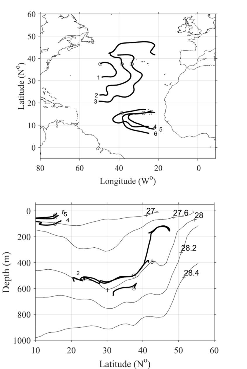
Figure 1 In the upper frame the Mercator projection and in the lower frame the meridional-depth projections of six ‘Preferred Trajectories’ (thick lines), three of them to signal the Subtropical Gyre and three of them the Subtropical Cell. The lower frame shows, in thin lines, contours of potential density referred to the surface at the longitude of 28° 30’ W. Both frames show the starting positions, with a small circle, for the integration of Eq. (12) (see Table I).

Conclusions
Multiple orthogonality constraints on the flow vector follow from the steady, non-diffusive, adiabatic, geostrophic and hydrostatic ocean model. The Boussinesq approximation is unneeded for such constraints. A pair of such constraints are Eqs. (8) and (11), which are related to: 1) the (ill-defined) ‘Neutral surfaces’ or conservation of ‘local’ potential density, and 2) the potential vorticity conservation set in the model defined by systems (2), (3) and (4). Compressibility effects and the Svedrup relation are essential in Eq.s (8) and (11). This pair of conditions produces a well-defined ‘local’ flow direction field (i.e., Eq. (12)), and, by integration, the ‘Preferred Trajectories’. Eq. (11) further restricts the ‘Neutral Paths’ (Bennett, 2019) of Eq. (8), hence producing individual, fully connected, ‘Preferred Trajectories’. We emphasize that: 1) the additional approximations to define and build global surfaces are, for the purpose of defining flow direction, unnecessary and 2) that this pair of constraints is closer to dynamical rules (i.e., to system (4)) than to thermodynamic rules (i.e., to systems (2) and (3)). The algebra, done in spherical coordinates, stresses the pertinence of the formalism to large-scale motions.

