


 nueva página del texto (beta)
 Inglés (pdf)
 Artículo en XML
 Referencias del artículo
 Enviar artículo por email
 Citado por SciELO
  Similares en
SciELO
Similares en
SciELO 
 Permalink
Introduction
The La Paz-Los Cabos region is an active tectonic zone with little historical seismicity reported, (Ortega and González, 2007). This article is a long-term effort, started in 1995 when a major earthquake struck the southern part of Baja California Peninsula. From 1996 to 1997 the Centro de Investigación Científica y de Educación Superior de Ensenada, Baja California (CICESE) deployed a local seismic network. Later, a temporary strong motion network was in operation from 1998 to 2007 (Munguía et al., 2006; Ortega and González, 2007). Recently, CICESE installed seismic broadband stations within and around La Paz Bay. For 15 years, seismicity and attenuation relations that are the basic parameters for seismic hazard analysis are been studied. In this work, a probabilistic seismic hazard analysis for the southern part of the Baja California Peninsula is presented.
Particularly, the seismic sources that have been a topic of active discussions are studied. There has been a long debate on whether some fault segments should be considered active or not. Of special importance are La Paz and San José faults because they are the most prominent features of the region. Therefore, all the fault segments that have been reported and mapped by the Mexican Geological Service (SGM, Servicio Geológico Mexicano) are presented. For example, some authors, (Cruz-Falcón et al, 2010; Munguía et al, 2006) have reported the existence of La Paz fault, whereas others, (Busch et al, 2006; Busch et al., 2007; Maloney et al., 2007; Ramos 1998) say this fault does not exist. In addition, a common problem is that there are several faults which cannot be identified with a unique name. The purpose of this work is to compare the seismic hazard in different scenarios: a) using all faults, b) without La Paz Fault (WLP) and c) without the San Jose Fault (WSJ). It is important to note that in this article active Quaternary faults only those faults that have exhibited an observed movement or evidence of seismic activity during the last 20,000 years are called.
Tectonic setting
The Gulf of California is an oblique - divergent plate boundary with active transtensional continental rifting (Busby and Ingersoll, 1995). Strike slip and normal faults systems accommodate the deformation in this region (Angelier et al., 1981; Fletcher and Munguía, 2000; Umhoefer et al., 2002; Plattner et al., 2007). Right lateral strike slip faults marked the extremities of the Gulf of California and they are separated by short spreading centers. On the east side of the southern part of Baja California peninsula an array of onshore to offshore faults north striking exists, left stepping and east dipping known as system of gulf margin (Fletcher and Munguía, 2000) (Figure 1).
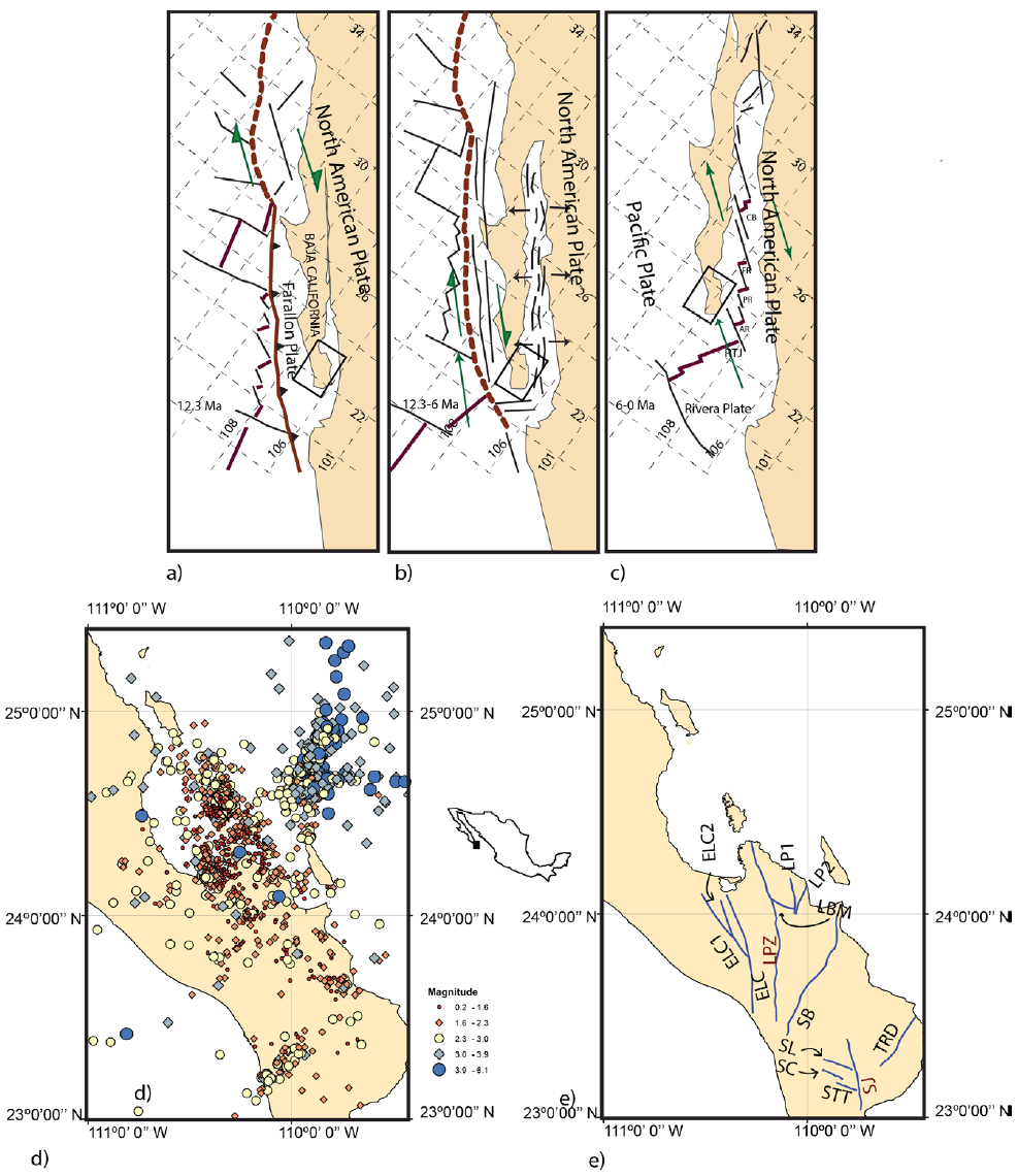
Figure 1 a) Farallon Plate that began the process of subduction starting the development of the Rivera Triple Junction. Between 20 and 12 Ma a series of microplates were formed along Baja California. b) Between 12 and 6 Ma normal faults with NNW and N trend, developed the east of the Tosco-Abreojos fault the system of normal faults was part of the distribution of the deformation, the gulf margin system was part of a complex system of transtensional faults. c) The regime of oblique divergence started about 6 Ma, when small rift basins began to form in the current Gulf of California. d) seismicity of the region, the complete catalog is represented. e) Quaternary Faults used in this article, La Paz and San José faults are used later to define different scenarios. AR, Alarcon Rise, PR, Pescadero Rise, FR Frallon Rise, CB Carmen Basin, RTJ, Rivera Triple Junction, and the faults: ELC, El Carrizal, ELC1, El Carrizal 1, ELC2, El Carrizal 2, LPZ, La Paz, LP1, San Juan de los Planes I, LP2, San Juan de los Planes II, LBM La Buena Mujer, SB, San Bartolo, TRD, La Trinidad, SL, San Lazaro, SC, San Carlos.
During the continental rifting (DeMets, 1995; Fletcher and Munguía, 2000; Plattner et al., 2007; Lizarralde et al., 2007), starts the onset of seafloor spreading in the southern part of the Gulf of California (Lizarralde et al., 2007); Umhoefer et al., 2008). In this region, the fault system development could be studied during the transition of rift to drift process, when ocean spreading begun and continental rifting is active. Along the Alarcon rise in the southern Gulf of California the spreading rate is slower than across plate boundary of the Pacific - North America, indicating that structures along with transform faults and spreading centers in the gulf could finally accommodate deformation in this region (DeMets, 1995; Fletcher and Munguía, 2000; Plattner et al., 2007).
The seismicity data (Munguía et al., 2006) and geomorphic relationships (Fletcher and Munguía, 2000; Busch et al., 2006, 2007; Maloney et al., 2007) show that the normal faults array rupturing the southern tip of Baja California peninsula are still active and act as a shear zone which contributes to translating the peninsula blocks away from mainland Mexico (Plattner et al., 2007). The gulf - border is an extensional zone as well as an area of decreasing elevation and thinning crust (Lizarralde et al., 2007). The topography of the southern tip of the Baja California peninsula is controlled by normal faults which produced moderate sized earthquake (Fletcher and Munguía, 2000), whereas the gulf margin fault array has a minor contribution to the plate divergence in the region. The faults delineate Quaternary basins and offset Quaternary alluvial deposits (Fletcher and Munguía, 2000; Busch et al., 2006, 2007; Maloney et al, 2007).
During the Cenozoic, the western part of North America at the latitude of Baja California was the place of a subduction zone, where Farallon plate was subducting beneath Western North America (Stock and Hodges, 1989; Hausback, 1984). During Farallon plate subduction (Figure 1a), the Pacific plate, located west of the Farallon plate met the North America plate (Atwater, 1970; Stock and Hodges, 1989) and stopped the subduction in the north beginning the development of the Mendocino and Rivera triple junction along southern California and northern Baja California (Gorbatov and Fukao, 2005).
While Mendocino triple junction moved northward the Rivera triple junction went southward lengthening the right lateral transform plate boundary that had initiated between Pacific and North America plates (Stock and Hodges, 1989). This right-lateral system developed marked the early stages of San Andreas system (Atwater, 1970). Between 20 and 12 Ma a series of microplates was formed along Baja California. The microplates were located within the Pacific Plate, and the trench was developed in a right lateral fault zone, known as the Tosco-Abreojos fault (Stock and Hodges, 1989). Between 12 and 6 Ma normal faults with NNW and N trend, developed the east of the Tosco-Abreojos fault (Figure 1b) adjacent to the west of the current Gulf region from California (Stock and Hodges, 1989; Hausback, 1984; Umhoefer et al., 2002). The system of normal faults that dominates the margin of the gulf was part of the distribution of the deformation between the Gulf of California and the Tosco-Abreojos fault (Stock and Hodges, 1989), the gulf margin system was part of a complex system of transtensional faults from 12 Ma (Fletcher et al., 2007). The regime of oblique-divergence started about 6 ago Ma, when small rift basins began to form in the current Gulf of California (Figure 1c). This oblique - divergence regime began as transform faults separated by rift basins (Fletcher and Munguía, 2000; Oskin et al., 2001; Fletcher et al., 2007). Along Alarcon Rise, the southernmost spreading center in the Gulf of California, new ocean crust started forming (DeMets, 1995; Umhoefer et al., 2008). Nowadays, the Gulf of California continues to be an oblique divergent continental rifting (Fletcher and Munguía, 2000; Umhoefer et al., 2002; Mayer and Vincent, 1999; DeMets, 1995).
Method
In this study, a classical approach for Probabilistic Seismic Hazard Analysis (PSHA) was used based on a three-step procedure (Cornell, 1968; Algermissen et al., 1990; Algermissen and Perkins, 1976; Bernreuter et al., 1989; Electric Power Research Institute, 1986). First, the seismicity parameters (a and b values) of the transform fault system were obtained. The Quaternary faults with low seismicity rate were also included using their annual rate of displacement obtained from independent studies. These faults were assumed to present a constant moment rate. Next, the attenuation relations were estimated using a simple omega-squared model based on a general regression of the maximum acceleration recorded versus distance. These attenuation relations for this region were published in a previous work (Ortega and González, 2007). Finally, the hazard maps were computed to show probabilistic ground accelerations with 10%, 5%, and 2% probabilities of excee-dance in 50, 100 and 200 years. The maps were constructed on the assumption that earthquake occurrence is Poissonian. Then the hazard curve was computed for three specific dams belonging to the National Commission of Water in Mexico and different fault system combinations comparing the results. The details on the hazard estimation are described in Frankel (1995), and Frankel et al., (1997). In the following sections, the steps to prepare the different parts of the probabilistic hazard analysis are describe.
Seismicity and moment rate
Two different models were used to compute the seismic hazard: Gutenberg-Richter and Characteristic Models. The former was used to analyze the transform fault system of the Gulf of California and the latter was used for the Quaternary faults within the Baja California Peninsula. For the Gutenberg-Richter model, the catalog was compiled for 18 years of operation of La Paz Seismic Network (Munguía et al., 2006). 2127 earthquakes ranging from 1 to 6.1 degrees in magnitude, between 23° < Lat < 25° and -111° < Long < -108° were located. The catalog to remove the aftershocks of 1998 in Los Barriles, and 2007 Cerralvo earthquake was reviewed (Ortega and Quintanar, 2010). In Figure 1d the seismicity of the region from 1998 to 2013 is present.
The a and b values were computed using the EMR method described by Woessner and Wiemer (2005), and coded in the Z-Map suite of programs (Wiemer, 2001, Figure 2). The b values were estimated using a maximum likelihood method (Bender, 1983).
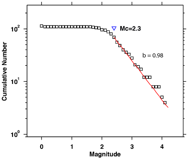
Figure 2 Plot of cumulative number of earthquakes versus earthquake magnitude, Mc =2.2 is the magnitude of completeness (b value is equal to 0.98).
The hazard calculation using the Gutenberg - Richter model involves the summation of the source contribution ranging from a minimum to a maximum expected earthquake magnitude. For each magnitude, a fault rupture length is calculated using the relationships of Wells and Coppersmith (1994). Next, a floating fault along the geological fault was set, and then the distance to the floating rupture for each site to calculate the frequency of exceedance (equation 2 from Frankel (1995) was found).
The estimation of the annual rate of earthquakes (v0) for a characteristic fault was computed using the following relation (Wesnousky, 1986, Stirling and Gerstenberger, 2018):
w here μ is the shear modulus (30 GPa), u the annual slip rate of the fault, L and W are the fault length and width, respectively and M 0c the characteristic moment obtained from the empirical scaling relation of Wells and Coppersmith (1994). The width of the fault W was determined assuming a seismogenic depth of 20 km and projecting its dip, so that the width is equal to 20 km divided by the sine of the dip. The fault length is calculated from the total length of the digitized fault traces (Figure 1b). The slip rate was estimated using paleoseismic studies based on the overall vertical offset of the basins, and quantitative studies using trenches in specific areas (Maloney et al., 2007). Table 1 shows inland faults displacements and other parameters useful to estimate (1).
Table 1 Quaternary fault parameters used in this study.
| No. | Length (km) |
Name | Mmax | Min. displacement (mm / year) |
Max. displacement (mm / year) |
Average displacement (mm / year) | Mo (dyne/cm) |
Moment rate (dyne/cm*year) |
|---|---|---|---|---|---|---|---|---|
| 1 | 19.3 | San Juan
de Los Planes I |
6.68 | 0.25 | 1 | 0.63 | 1.17E+26 | 7.24E+22 |
| 2 | 16.09 | San Juan
de Los Planes II |
6.61 | 0.25 | 1 | 0.63 | 9.22E+25 | 6.03E+22 |
| 3 | 13.42 | La Buena
Mujer |
6.54 | 0.25 | 1 | 0.63 | 7.27E+25 | 5.03E+22 |
| 4 | 39.47 | San José
del Cabo |
6.95 | 0.5 | 1.5 | 1.00 | 2.97E+26 | 2.37E+23 |
| 5 | 15.22 | San Lázaro | 6.59 | 0.5 | 1.5 | 1.00 | 8.57E+25 | 9.13E+22 |
| 6 | 11 | Saltito | 6.47 | 0.7 | 0.8 | 0.75 | 5.61E+25 | 4.95E+22 |
| 7 | 11.35 | San Carlos | 6.48 | 0.25 | 1 | 0.63 | 5.84E+25 | 4.26E+22 |
| 8 | 71.4 | San Bartolo | 7.17 | 1 | 1 | 1.00 | 6.44E+26 | 4.28E+23 |
| 9 | 32.9 | Trinidad | 6.88 | 1 | 1 | 1.00 | 2.34E+26 | 1.97E+23 |
| 10 | 100 | La Paz | 7.30 | 0.11 | 1.6 | 0.86 | 1.00E+27 | 5.13E+23 |
| 11 | 65 | Carrizal | 7.14 | 0.11 | 1.6 | 0.86 | 5.70E+26 | 3.33E+23 |
| 12 | 34 | Carrizal1 | 6.89 | 0.11 | 1.6 | 0.86 | 2.45E+26 | 1.74E+23 |
| 13 | 37.5 | Carrizal2 | 6.93 | 0.11 | 1.6 | 0.86 | 2.78E+26 | 1.92E+23 |
The characteristic magnitude was determined from the length of the fault using the relationships of Wells and Coppersmith (1994), whose regression parameters depend on the tectonic environment. The characteristic moment was finally calculated from Kanamori (1977) equation once given the characteristic magnitude.
Attenuation relations
The earthquake attenuation relations estimated in this area by Ortega and González (2007) were used. They observed that the attenuation in general is similar to that of southern California. The data were recorded using 32 strong-motion seismic stations from La Paz network (LAP) comprising 1320 small to moderate earthquakes (Figure 3). Some characteristics of the ground motion are:
a) ttenuation functions for distances ranging between 40 and 100 km tend to slightly increase their amplitudes due to the critical reflections of the shear waves from the Moho. This feature is better observed at low frequencies (<5 Hz). These fluctuations are modeled in the parametric form of the geometrical spreading function, g(r), which controls some changes in the seismic wave propagation.
b) values of the geometrical spreading control the general propagation effect due to distance between site and source. This propagation effect includes the source parameters, effects from finite faults that generate seismic waves at different depths, and the contribution of small and large earthquakes.
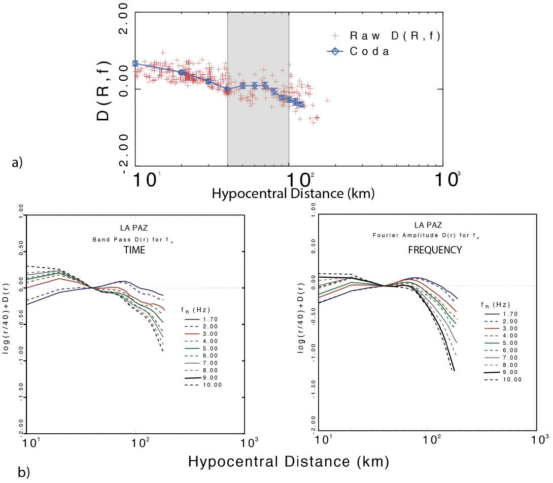
Figure 3 Attenuation relations estimated in the area. Top, example of the attenuation function from the regression, the gray area represents the distance between 40 and 100 km where the geometrical spreading exponent is low (0.2). Bottom, attenuation function for different frequencies using time (left) or frequency (right) analysis.
The predicted ground motion spectra at a frequency f as a function of the hypocentral distance r is given by:
where:
and, S(f,M w ) is the source Fourier velocity spectrum
M w is the moment magnitude
g(r obs) is the geometrical spreading function relative to r obs = 40 km
Q(f) is the frequency-dependent quality factor
β is the shear-wave propagation velocity
κ eff is a site attenuation coefficient
r obs is the observed distance from which we extrapolate to other distances
The second term is a level of motion that propagates the S(f, M w) term at r obs. The source function S(f) is a simple ω2 modeîas described by Brune (1970):
where:
C is equal to (0.55) (2) (0.707)/4πρβ3 the term [4.91×10⁶ β(Δσ/M0 ) 1/3] is the corner frequency
Δσ is the stress parameter in (bars)
β is the average shear-wave crustalvelocity (3.5 km/sec.)
M0 is the scalar seismic moment, which in turn is related to the moment magnitude (Kanamori, 1977).
Magnitude-distance tables were constructed using the SMSIM suite (Boore, 1983) and the ground motion parameters of Table 2.
Table 2 Ground-motion parameters
| K eff | 0.06 |
| Q( f ) | 180f0.32 |
| β | 3.5 |
| ρ | 2.8 |
|
|
GEN97* |
| Δσ | 40 |
| G(r) |
|
These attenuation relations are used in a look-up table procedure that was originally coded by (Frankel, 1995) in the USGS computer programs.
Hazard estimation
The hazard calculation was performed using the codes of USGS for the National Seismic Hazard Mapping Project (NSHMP) (Petersen, 2008). This code has the flexibility to be easily adapted and has been extensively reviewed during some decades (Frankel, 1995; Frankel et al, 1997). The attenuation relation's analysis were adapted using a look-up table. This code has the advantage that the data structure is virtually identical to the New Generation of Attenuation relations (NGA) that has been reviewed recently. So, any logical tree that would be adequate to this region can be created, including NGA attenuation relations. For simplicity, the attenuation relations of Table 2 were used. On the other hand, there are some advantages of using this computer code such as simple input of geological data and easy access to adjust the source code. This code has different modules including a smoothed grid source (Frankel, 1995) and floating fault sources. The program allows choosing between Gutenberg - Richter or the Characteristic models. During the last 20 years, thas been observed that there is not enough information to compute robust a and b values for Quaternary faults. However, for transform fault systems, the Gutenberg - Richter model is adequate. Most of the seismicity occurred in main - aftershock earthquake sequences, and once the aftershock removal is performed, the seismicity parameters can be obtained. The hazard calculation was performed using the Characteristic model for the Quaternary faults and the Gutenberg - Richter for the transform fault system.
Fault contributions
There are two types of sources. Active faults and Quaternary Faults both sources are fault areas; there is much work in defining the correct source. For the Quaternary faults, which is the focus of this article, in a map view, a fault is a line because it is expressed as a strike and dip. Not a smoothed grid area source was used because the transform system is well defined and there is no sparse seismicity in the surrounding region. The active faults were modeled using the Anderson (1979) model. The seismogenic thickness is constrained to 20 km; the fault dip is based on geophysical models (Arzate, 1986). Since the present model is based on the Characteristic fault rupture, then completeness magnitude and statistical values of a and b are not used. However, in the active tectonics, the maximum magnitude and magnitude range play an essential role.
In the study area, faults that control the hazard are not well identified and different authors disagree on whether some faults should be considered as potentially dangerous in hazard estimation. The purpose of this work is to test whether there are significant differences if some Quaternary fault segments are included or discarded in the seismic hazard analysis. First, the seismic hazard was computed using all the source information that is available from the national geological maps of the Mexican Geological Survey (SGM), using the 1: 10,000 and 1: 250,000 maps (SGM, 1996, 1999, 2000, 2001, 2002, 2008). Second, two different scenarios were computed: scenario (a), the seismic hazard without La Paz fault (WLP), and scenario (b) seismic hazard without San Jose fault (WSJ). Finally, the PGA for 3 sites was computed. In Figure 4, the results of the probabilistic seismic hazard analysis for all the faults are shown. It is noticeable that the Transform Fault System of the Gulf of California controls the seismic hazard for short return periods. This are to the use of the Characteristic Model for inland faults with a return period greater than 1000 years, and these characteristic faults do not contribute to the hazard estimation for short return periods. On the other hand, in the case of long return periods the characteristic faults control the hazard.
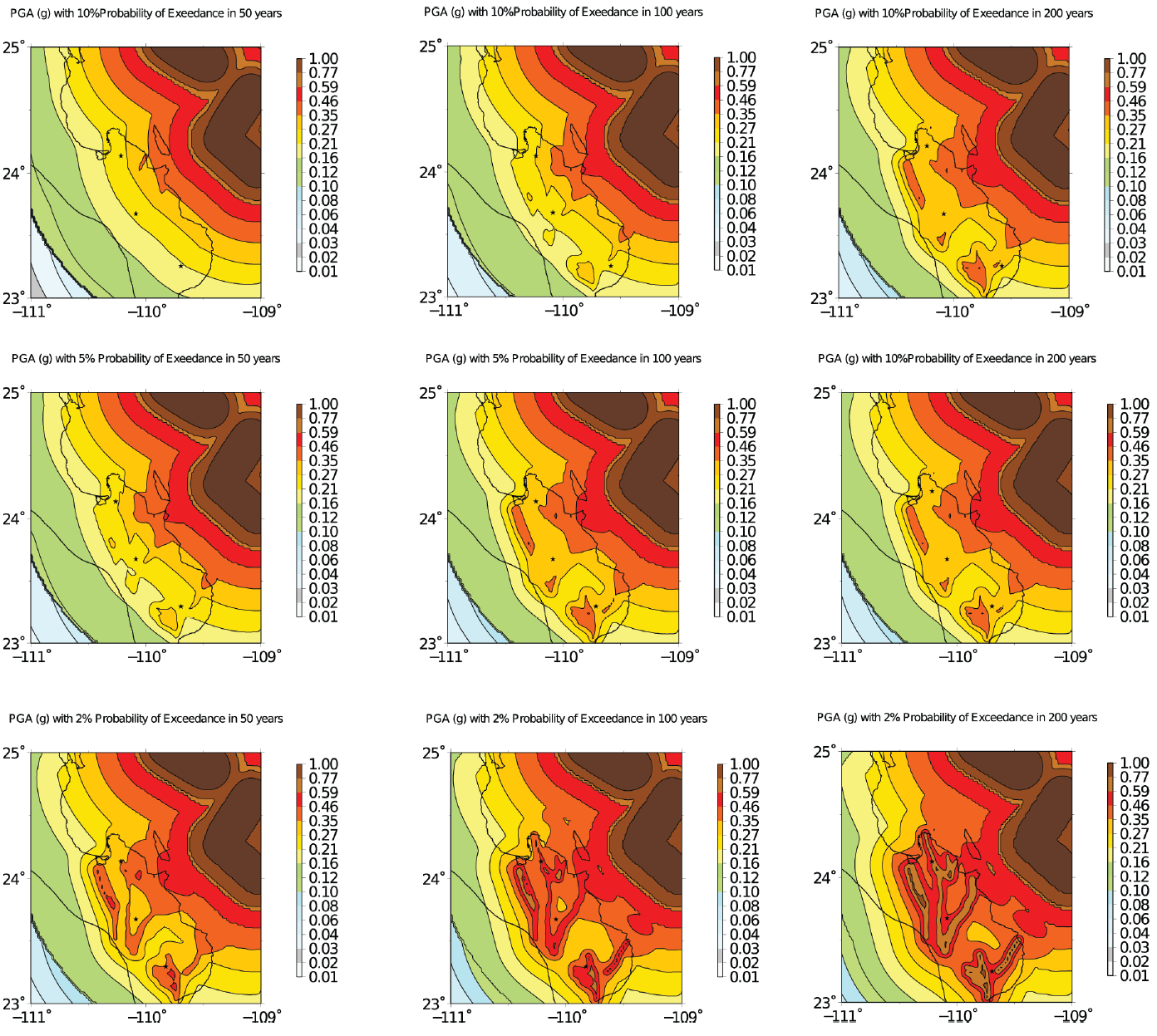
Figure 4 Probabilistic seismic hazard analysis for different return periods and observation times using all the sources. The transform fault system is located at the top right of the map and analyzed with the Gutenberg-Richter model. The Quaternary faults are located within the Baja California Peninsula and analyzed with the Characteristic model, the stars represent the site of the dams, the northern dam is La Buena Mujer, in the middle Santa Ines and at the southern side La Palma (see text for details).
In Figure 4, the lower panels represent the 2% of exceedance of 50, 100 and 200 years that correspond to return periods of 2479, 4950 and 9900 years, respectively. These return periods are usually used for the engineering design of essential facilities such as bridges and dams.
In the last panel of Figure 4, the location of the three principal dams (stars) match with the region of the high seismic hazard.
In Figure 5 the seismic hazard using the WLP model is shown and for short return periods (panels 1, 2, 4) the maps are virtually identical. However, for long return periods there are substantial differences among the principal dams, especially for the Buena Mujer and Santa Ines dams, identified at the northern side of the region (panels 6, 7, 8 and 9). In contrast, La Palma dam is too far from La Paz fault and the hazard contribution is negligible.
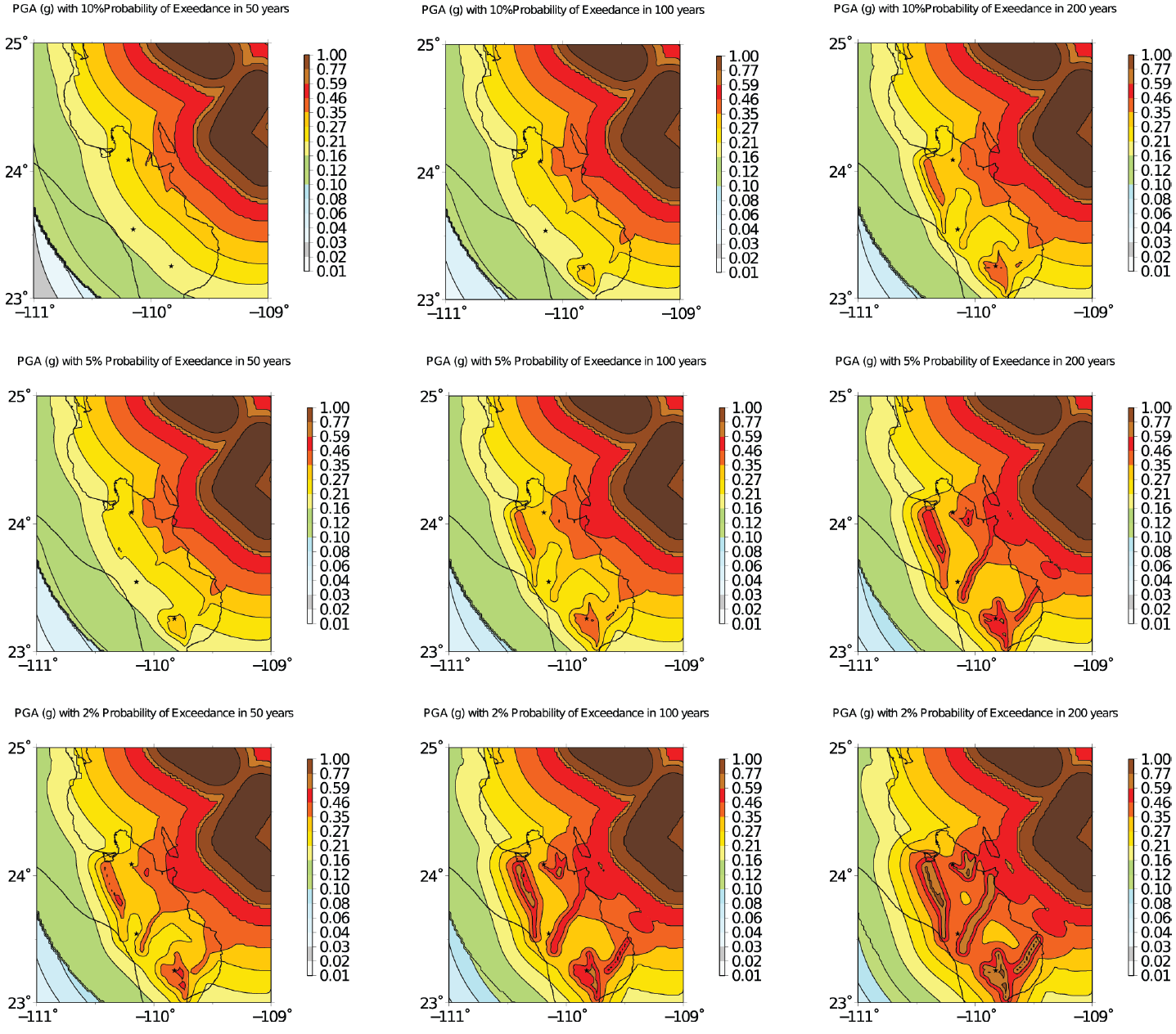
Figure 5 Probabilistic seismic hazard analysis for different exceedance probabilities and observation periods using the WLP model. The transform fault system is located at the top right of the map and analyzed with the Gutenberg-Richter model. The Quaternary faults are located within the Baja California Peninsula and analyzed with the Characteristic model (see text for details).
Similarly, in Figure 6, the hazard using the WSJ model was calculated. The San José fault affects La Palma dam and is not contributing to the hazard of Buena Mujer and Santa Ines dams. In this case, the presence of smaller faults (Saltito, San Lazaro, Trinidad) are of special importance since they are located close to La Palma dam and the absence of the San José fault in the hazard calculation is not so sensitive as is the case of the WLP model.
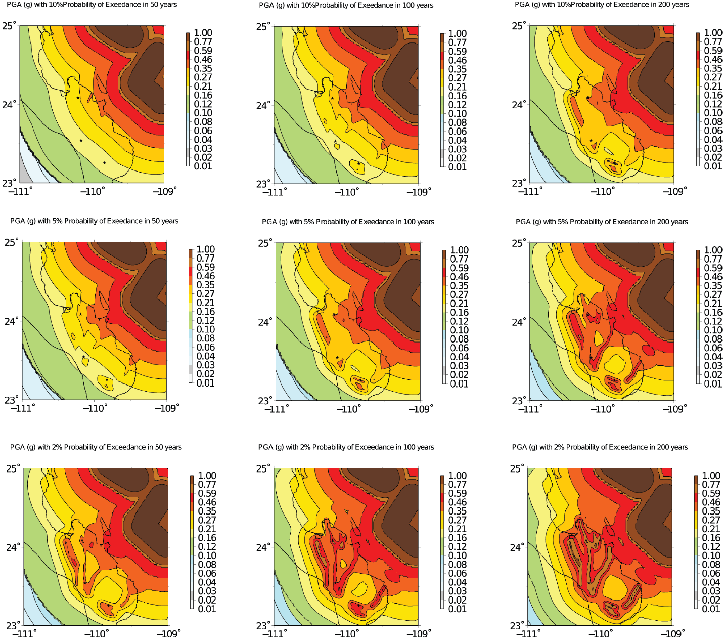
Figure 6 Probabilistic seismic hazard analysis for different return periods and observation times using the WSJ model. The transform fault system is located at the top right of the map and it was analyzed with the Gutenberg-Richter model. The Quaternary faults are located within the Baja California Peninsula and analyzed with the Characteristic model (see text for details).
Figure 7 shows a comparison among models for PGA values of hazard calculation for different return periods and the three different fault scenarios. In the absence of these faults, the PGA is reduced for the long return period.
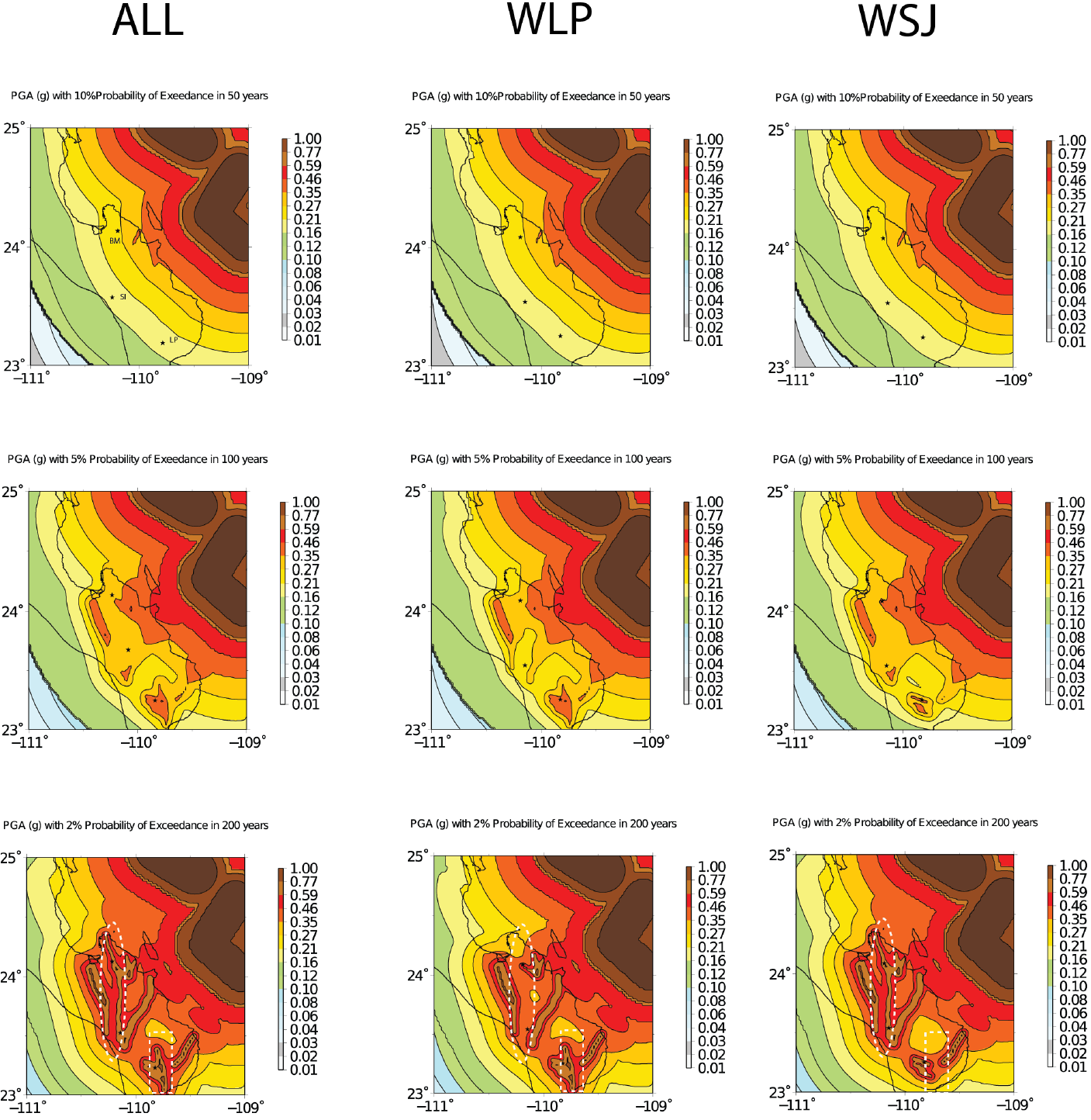
Figure 7 Contour plot for PGA values of hazard calculation for different return periods and three different fault scenarios. Left column, model with all faults; central column, model without La Paz fault; right column, model without San José fault. The cases are 10% of probability of exceedance in 50 years (first row, from top to bottom); 5% of probability of exceedance in 100 years (second row); 2% of probability of exceedance in 200 years (third row). The last row shows the long return period expressed as 2% probability of exceedance in 200 years. The elliptical region covers La Paz fault and the squared region San Jose fault. BM Buena Mujer Dam, SI Santa Ines Dam and LP La Palma Dam.
In Figure 8, the hazard curve of the complete model for La Palma, Santa Ines and Buena Mujer dams is depicted. In the hazard curve, the Characteristic Fault Model was used excluding the transform faults of the Gulf of California. The three curves are similar; the Buena Mujer and Santa Ines curves are parallel because their hazard is controlled mainly by La Paz fault, and the rest of the faults are not important.
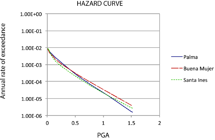
Figure 8 Hazard curve for the complete model for La Palma, Santa Ines and Buena Mujer dams using the Characteristic models of the Quaternary faults.
In Figure 9, the hazard curves of the three dams using the WLP model are shown. In this case, the three curves are different and we observe that the Santa Ines dam has lower PGA values. The Santa Ines dam is relatively far from the other faults, except for La Paz fault that is the closest to the dam.
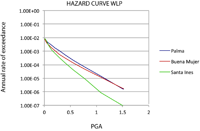
Figure 9 Hazard curve of the WLP for La Palma, Santa Ines and Buena Mujer dams using the Characteristic models of the Quaternary faults.
In Figure 10, the WSJ model is depicted. Interestingly, the WSJ and the complete model of Figure 8 are similar, suggesting that for these sites the contribution of the San José fault is not so important.
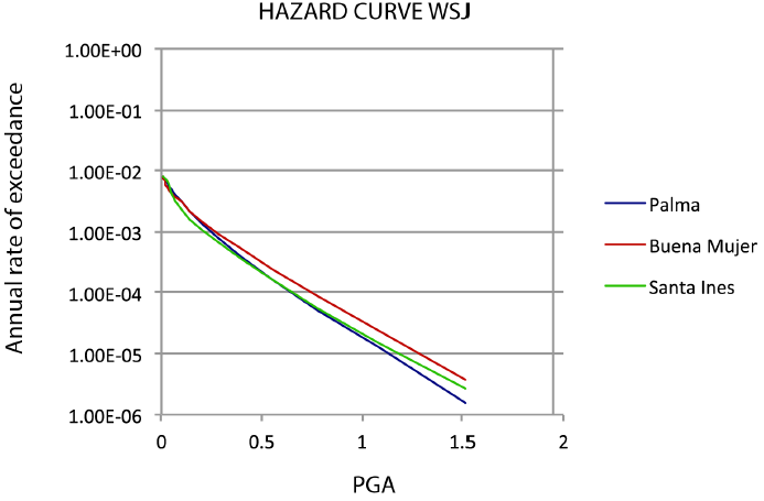
Figure 10 Hazard curve of the WSJ for La Palma, Santa Ines and Buena Mujer dams using the Characteristic models of the Quaternary faults.
In general, the hazard estimation has been used in Mexico with a and b values statistical coefficients of seismicity. Little importance has been given to faults that exhibit large return periods and pose risks in the long term. A recent example reported by a study of seismic hazard in central Mexico used instrumental seismicity as well as historical data includeding fault information (Beyona et al., 2017). However, this is the first time that a similar study is performed in Baja California Sur. There are some reasons why long return periods have not been traditionally considered in the seismic hazard estimation in Mexico, such as: a) the high active tectonics in the coast which is usually more important than inland active faults and b) there are insufficient paleoseismic studies in the region. However, in Baja California Sur, the active sources with high annual moment rate occur in the Gulf of California, and Quaternary faults are located in the peninsula. Moreover, this region was originally populated in areas close to principal faults, because these faults are the principal sources of water that is collected from the mountain ranges situated at the center of the Peninsula. Also, these faults are the cause of the high mineralization of gold, copper and silver, giving rise to important mining development. Therefore, there is a high correlation between fault location and population.
Another contribution of this study is the usage of attenuation relations obtained for this region. A simple look-up table of magnitude-distance based was introduced on the work of Ortega and González, (2007). However, the results do not differ considerably when the attenuation relations of Southern California are used instead, since they are characterized by similar values of Q(f), geometrical spreading function and kappa (Ortega and Gonzalez, 2007). Moreover, the NGA attenuation relations are also a good approximation. In this work, rather than analyzing the sensitivity of the predictive relationships, the differences in considering or ignoring some faults are studied.
Discussions
Including or excluding faults in PSHA implies great differences in the results. This is not surprising in PSHA because this problem has been observed over decades in different regions, however, there are some interesting aspects of this region that we will discuss. First, the PSHA is based on a formal probabilistic framework that considers all the uncertainties, including the epistemic ones. For this reason, PSHA is based on logic trees that mimics the probability distribution of the seismic sources epistemic errors. To design the logic tree, decisions are always made through panels of experts. Marzochi and Jordan (2017) discussed a global framework to analyze the PSHA, in their article they noted the importance of the participation of experts, but it is important to say that there is a subjective part that implies adding preferential information, which not always seem to have a scientific basis. It is important to emphasize that adding subjective preferences is not necessarily non-scientific knowledge, the most important thing is to be able to prove if our preferences make sense or if they should be discarded in the future.
A problem that frequently occurs in the PSHA by participating in a committee of experts that is specifically focused to seismic hazard, is that experts tend to strategically manipulate their opinion. For example, in the case of giving advice on the existence of a fault to develop hazard maps, an expert knows that in case of an error there is a risk of a major disaster, but in the case of developing maps of natural resources those errors are not so relevant and probably their opinion will be different. In addition, an expert may be pro- environment and inadvertently he would include more restrictions if the panel of experts take decissions for nuclear power plants for example. After analyzing the best option for PSHA the logic tree of Figure 11 was prefered. This model exemplifies the epistemic uncertainty of sources, magnitude and attenuation relations (GMPE, Ground motion prediction equations).
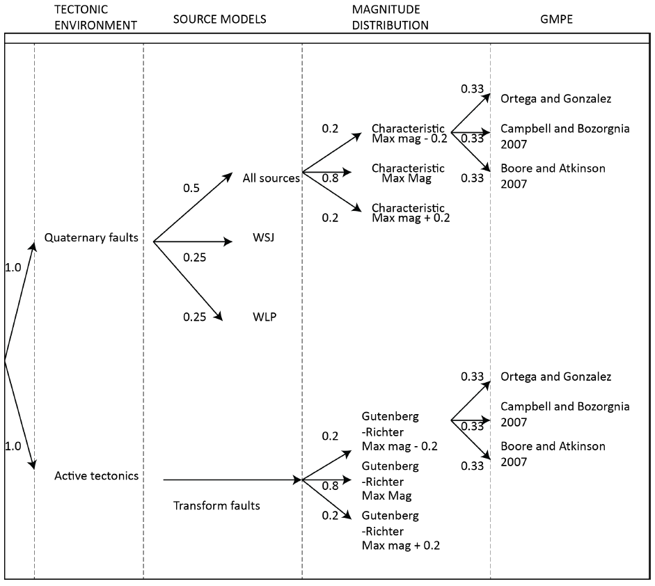
The logic tree of Figure 11 is based on analyzing advantages and disadvantages of the different models. In this model, the most important decision was the Quaternary faults weights of three different models (all faults, WSJ and WLP).
In Figure 12 the final map for two return periods is presented, the first panel represents 2% of exceedance in 50 years, the second represents 2% of exceedance in 200 years, therefore the first is equivalent to a return period of 2475 years and de second of 9900 years. In this interval, there is a major difference in the hazard maps. However, the 2475 return period is sometimes considered as the highest threshold for essential facilities. Comparing the 2475 return period (Figure 12 first panel) with the 474 years (Figure 4 first panel) we observe that the Quaternary faults apparently are not sensitive for high rates. However, this is only a mere artifact of the arbitrary decision of using return periods as a degree of protection because at higher return periods the hazard should be nuanced. Recently Stirling and Gerstengerg (2018), studied the applicability of a Gutenberg-Richter magnitude distribution instead of the Characteristic fault model. In their study Stirling and Gerstengerg (2018) analyzed active faults with high slip rates (> 1 mm/yr), their results suggest that the Gutenberg Richter magnitude distribution is compatible with active faults and cannot be ruled out in PSHA, but for low slip rates ( < 1 mm/yr), this possibility has not been tested yet. Our study opens a possibility to improve the PSHA in Baja California to include the Gutenberg-Richter magnitude distribution in the future. Similar studies have been reported in central Mexico (Bayona et al., 2017). Work is in progress to present a combination of Gutenberg-Richter and Characteristic magnitude distribution. Care should be taken if we compare our results with other studies, for example, it is common to represent a PGA concerning a specific rock site namely Vs30=760, this reference is based on geotechnical studies in which there is a competent rock at 30m depth with a value of 760 m/s for shear wave velocity. We used a general average value that represents the common amplification of the basins in BCS. Also, we used a low attenuation model. It is important to note that we do not have the intention to use our results for engineering purposes until we can validate them.
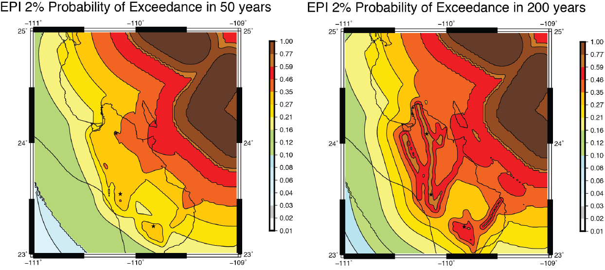
Figure 12 Hazard map of the final model using a logic tree for Baja California Sur for two different return periods. The 2% probability of exceedance in 50 years is a standard for dam designs. In contrast a 2% probability of exceedance in 200 years is plotted for comparison.
This article reflects the importance of studying active Quaternary faults at a regional scale. Paleoseismic studies provide valuable information about slip rates. It is crucial to use this information in the seismic hazard analysis and include the results in a specific way that can be useful in hazard maps. For example, Busch et al. studied the Carrizal Fault (Figure 1) they prepared trenches and presented their results in a self-consistent tectonic framework. Their studies discussed a tectonic relation of the transtensional regime in Baja California. We obtained the slip rate from their analysis, but in other cases, the slip rate is not estimated. For example in the La Paz fault. In that case, we only estimated a possible slip rate based on limited work about the fault.
Nowadays, paleoseismology studies are becoming a new discipline; they also provide information that the instrumental seismicity is not capable of obtaining. The active crustal faults sometimes are not included in PSHA because it seems that they are not as dangerous if compared to active tectonics (e.g., subduction margins), but we believe that this impression is incorrect. The Major-Cucapah earthquake in 2010 (Mw = 7.2) that occurred in Mexicali, Baja California is an excellent example of a crustal fault that caused severe damages. The geological and geophysical geometry is essential to consider in mapping the damages (Wei et al., 2011), the recurrence is about 2,000 years (Rockwell et al., 2010) so, if we compare to the active tectonics of few tens of years, it probably should be not so critical. However, the problem is the location of these faults. In the Baja Peninsula, the faults are located close to the urban centers.
Another problem to address is the lack of studies and instrumentation. For example, Suter (2018) reported the Loreto earthquake of 1878; this event seems to be the worst scenario for Baja California Sur, the destruction was very severe. Up to date, there are no studies that identify the actual fault. Note that in this region, there are seismic records with extreme levels of PGA, in 2007 a strong motion instrument recorded an earthquake with a maximum value of 0.6 g in Bahia Asuncion (Munguia et al., 2010; Ortega et al., 2017). The value of 0.6 g exceeds by far any expected value in previous hazard maps in the region, reflecting the need to study the Quaternary Faults and the effect in the seismic hazard.
We conclude that the Quaternary faults are only important when computing the hazard using high recurrence rates. In places where the active tectonic sources, such as faults belonging to the transform fault system, are far from the sites, as is the case of Baja California Sur, the contribution of the hazard of such Quaternary faults is not so evident. Specially for low recurrence rates. Clearly, a detailed paleoseismic study is of crucial importance to assess the hazard for this region. The complete model with all the sources is the best for earthquake-resistance structures, especially for dams' design. On the other hand, overestimating the hazard may have the consequence of introducing unnecessary severe construction codes causing an economic impact on the development of this region due to the increase in construction costs. In Mexico, there is no specific guidance for choosing return periods on dams' designs. However, the general trend of 2% of exceedance in 50 years may be not adequate and 2% of exceedance in 200 years seems to be adequate in Baja California Sur. This level of security has a large impact in the economic development and is very important for strategic planning.
Conclusions
The general conclusions are:
1) The southern part of Baja California is a region with important faults that control the seismic hazard of the high return periods.
2) Active Quaternary faults need to be studied, especially the average displacement or moment rates.
3) Specifically, in Baja California Sur, the return period for critical facilities should be 9900 years expressed as the 2% probability of exceedance in 200 years.

