


 nueva página del texto (beta)
 Inglés (pdf)
 Artículo en XML
 Referencias del artículo
 Enviar artículo por email
 Citado por SciELO
  Similares en
SciELO
Similares en
SciELO 
 Permalink
Introduction
Nowadays new techniques called Enhanced Oil Recovery Methods (EOR) are applied to improve the oil recovery in a hydrocarbon reservoir. Lake (1989) gives a definition for the EOR methods: EOR is oil recovery by the injection of materials not normally present in the reservoir. This definition covers all modes of oil recovery and most oil recovery agents. Considering this definition the EOR methods might consider both secondary and tertiary recovery. Before EOR methods are applied there is a technique that almost always has to be considered, that is, the waterflooding technique. Waterflooding technique is the oldest assisted recovery method and it remains as the most common method used to sweep the oil that was not produced by natural pressure, and to keep the oil pressure when this has declined due to reservoir conditions (Latil, 1980).On the other hand, due to the growing need in the oil industry to make faster and more efficient calculations to simulate the recovery conditions before, during and after the production life of a reservoir, it is necessary to test new computational techniques that reduce the run time of the numerical simulators. Several investigations have been carried out to improve the run time of the reservoir simulators (Killough et al., 1991; Shiralkar et al., 1998; Ma and Chen, 2004; Dogru et al., 2009). Most of these papers have been developed using distributed computing. Recently, Wang et al. (2015) developed a scalable black oil simulator using ten millions of grid blocks approximately, their simulator reached a scalability factor of 1.03 using 2048 processors. Also Liu et al. (2015) developed a three phase parallel simulator applying MPI (Message Passing Interface) for communications between computational nodes and OpenMP for shared memory. They obtained an efficiency of 95.7% by using 3072 processors. However, there is a limitation to use this technique, since a computational cluster with tens until thousands of processors is needed to achieve the desired speed up.
As an alternative NVIDIA has developed a programing language called CUDA (Compute Unified Device Architecture) which can be used to take advantage of the power computing graphics cards for general purpose simulations. Yu et al. (2012), used GPUs to parallelize a reservoir simulator which can run large scale problems. They used over one million grid blocks obtaining a good speed up compared to the numerical code of the CPU. Li and Saad (2013), developed a numerical code of preconditioned linear solvers based on GPU, their numerical experiments indicate that Incomplete LU (ILU) factorization preconditioned GMRES method achieved a speed up nearing to 4 compared versus CPU numerical code. Liu et al. (2013), reported improved preconditioners and algebraic multigrid linear solvers applied to reservoir simulations using GPUs. De la Cruz and Monsivais (2014) developed a two phase porous media flow simulator to compare the performance of a single GPU with a single node of a cluster using distributed memory. These authors found that a single GPU is better than a computational node with twelve processors. Trapeznikova et al. (2014) developed a software library for numerical simulation of multiphase porous media flows that is applied to GPU-CPU hybrid supercomputers. The model is implemented by an original algorithm of the explicit type. An explicit three-level approximation of the modified continuity equation is used. After that the Newton method is used locally at each point of the computational grid. Authors used SPE-10 project as benchmark, they achieved a 97x of speed up when they compare the run time obtained by a single GPU versus one CPU, and 18x of speed up when a computational node of six processors is used. Mukundakrishnan et al. (2015), presented the implementation in GPUs of a black oil simulator, which uses a fully implicit scheme for the discretization in the time and the constrained pressure residual -algebraic multigrid (CPR-AMG) to solve the linear system equations. They reported an average of 20 minutes for the run time to solve a problem with 16 million of active blocks by using 4 GPUs. Anciaux-Sedrakian et al. (2015) made a numerical study of different preconditioners such as: Polynomial, ILU and CPR-AMG which were implemented in a heterogeneous architecture (CPU-GPU). They emphasize two key points to obtain high performance in heterogeneous architectures; the first is to maximize the utilization and occupancy of the GPU and the second refers to minimize the high cost of transferring GPU data to the node with the CPUs and vice versa. Their results show that a combination of 1 processor plus 1 GPU is approximately 2 times faster compared versus an 8-processor node by applying CPR-AMG preconditioner.
In this work a simulator for oil recovery was developed based in the water injection process and the simultaneous solution technique described by Chen et al. (2006). A parallelization scheme is proposed by using GPUs for both the construction of the Jacobian matrix and the solution of the linear system of equations.
The paper is organized in this way: In Section 2, the mathematical equations of the water injection and pressure-saturation formulation model are introduced. In Section 3, the numerical discretization is presented by using the Finite Volume Method (FVM) and the linearization of the equations by applying the Newton-Rapshon method (NR). In Section 4, the computational implementation of the CPU and GPU are shown and main algorithms are explained. In Section 5, numerical results of three benchmark problems are presented. Also in this section, the performance of the parallel numerical code is evaluated by comparing the run time obtained in both GPU and CPU.
Mathematical model of the incompressible two-phase flow in porous media
The mathematical model of the incompressible two-phase flow can be used to simulate the water injection into a hydrocarbon reservoir. The mass balances are obtained by taking into account two phases: oil and water. Governing equations can be obtained by applying an axiomatic formulation (see Herrera and Pinder, 2012 for a complete description on this formulation). A general local balance mass equation can be written as follows:
Here ϕ is the porosity of the media ρα, S α, u α, and q α represent the density, saturation, velocity and source of phase α. The Darcy’s velocity is used expressed as follows:
where
The mass balance equations are interrelated by the following mathematical expressions:
where p
α is the pressure of the phase α,
Equations (3) and (4) are non-linear and strongly coupled. In order to simplify the numerical solution of these equations, the pressure-saturation formulation was used which consists in selecting oil pressure and water saturation as primary variables and in using the fractional flow theory to derive one equation for pressure and one equation for saturation (Peaceman, 1977; Chen et al., 2006). The mass balance equation for water phase is:
Considering non-compressible flow, equation (9) becomes:
where the following substitutions were carried out:
Taking into account the fractional flow of the phase α (f
α) that is defined as the quotient of the phase α mobility (λα) over the total mobility
For more details about fractional flow formulation readers can consult Chen et al., 2006. Considering no change in the porosity, and non-compressible flows, equation (13) can be reduced to:
Equations (10) and (14) are coupled and non-linear. The Newton-Raphson approach was used to linearize the equations and solve them using a fully-implicit strategy. In this work three different cases of study are described.
Numerical model
In this section a brief description is given of the use of the Finite Volume Method (FVM) to discretize equations (10) and (14), and the Newton-Raphson method to linearize those equations.
Calculation of residuals by using the Finite Volume Method
As a way to show how FVM is applied to compute the residuals for the governing equations, the saturation equation for the three-dimensional case is discretized. Integrating equation (10) with respect to time and the control volume shown in Figure 1, equation (15) is obtained:
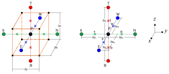
In order to evaluate the terms of equation (15) the following considerations were taken into account: 1) a backward Euler approximation is used, 2) the permeability tensor is diagonal and 3) the space derivatives are approximated using central differences. Therefore, the discretized form of equation (15) in terms of a residual is written as follows:
where the transmissibility is computed as
Here T i , implies the calculation of the transmissibility considering the total mobility λ and T w,i refers to the transmissibility considering the mobility of the water phase λ w . In equations (16) and (17) the superscript n + 1 is omitted for simplicity.
Newton-Rapshon Method
Because there are nonlinearities in the discretized equations, the Newton-Raphson method was selected to linearize and to solve these equations. The main advantage of the method is its numerical stability compared with methods which use explicit discretization (Abou-Kassem et al., 2006; Chen, 2007). For applying the Newton-Raphson method
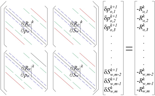
Matrix on the left of equation (18) is the Jacobian and superscript k is used to indicate the Newtonian iteration. The system written in extended form gives:
Equations (19), (20) along with the residuals (16) and (17) are used to build the linear system as shown in Figure 2, where the subscript m refers to the total number of discrete volumes.
One of the main issues in this kind of problems is how to calculate the Jacobian elements and how to solve the resulting linear system. Both tasks are time consuming, therefore new techniques are needed to reduce the time used in doing these computational processes. In the next section details of the computational implementation that makes use of graphical processing units (GPUs) are presented in order to parallelize the construction of the Jacobian and the solution of the resulting linear system
Computational implementation
In this section, the computational methodology used is briefly described to implement the algorithms provided by the numerical methods outlined in previous sections.
CPU Implementation
First of all, the algorithms to be executed in an ordinary CPU were implemented for comparison purposes. The codes were written using the C++ language and the EIGEN library (Jacob and Guennebaud, 2016), the last one was used to simplify the array and matrices management and the solution of the linear systems of equations. The pseudocode of the main algorithm is shown in Figure 3.
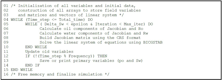
In the first three lines of the pseudocode shown in Figure 3, all required variables and arrays are declared and initialized with adequate values, this includes the initial and boundary conditions, petrophysical values, size of the mesh, time step, etc. In line 4 the simulation initiates and is carried out until the total number of time steps is reached. Inside this first cycle, another one implements the Newton-Raphson (NR) algorithm. This internal cycle starts in line 5 and is carried out until the norm of the change of the water saturation (∣δS w ∣) is less than a prescribed value (ε) or the prescribed maximum number of iterations of the NR algorithm is reached. Lines 6 to 9 represent the main steps to solve the problem and use the highest percentage of CPU time. In lines 6 and 7 every entry of the Jacobian matrix is calculated, this means to calculate the discretized components of the residuals, equations (18) and (19), and their corresponding derivatives. It is worth mentioning that all derivatives are done numerically and first order forward finite differences are used to do so. Then in step 9 the Jacobian matrix is build using the Compressed Row Storage (CRS) format in order to take advantage of the sparseness of the matrix and to save memory. In the calculations, these three steps take around 8% of the total time. In line 9 the linear system is solved using the Biconjugate Gradient Stabilized (BICGSTAB) method algorithm which is contained in the EIGEN library. This step takes around 75% of the total CPU time. Once the NR algorithm has converged, all the required variables were updated to be used in the next time step, line 11. Finally, the solution (primary variables) were saved or printed every time the Iteration variable is divisible by a prescribed Frequency. This frequency will become important in the GPU implementation.
GPU Implementation
The implementation in CPU presented in the previous section is standard and do not have any complications. For the GPU implementation the Compute Unified Device Architecture (NVIDIA, 2012) and the CUSP Library were used, which provides a high-level interface for manipulating sparse matrices and solving sparse linear systems (Maia and Dalton, 2016). The present implementation is almost done totally in GPU, which means that the amount of information exchange between CPU and GPU is relatively low. In this sense, the pseudocode of the main algorithm for GPU implementation is similar to the one shown in Figure 3. The following differences have to be mentioned: a) the cycle starting in line 4 require all the variables and arrays defined in lines 1-3, therefore a first exchange of information is done from CPU to GPU, however this is minimal due to the fact that the biggest arrays are constructed directly in the GPU; b) the operations in lines 6, 7, 8, 9 and 11 are all coded in CUDA, therefore, several kernel functions occur that are executed in the GPU device; c) the operation in line 13 requires a movement of information from GPU to CPU, however this is done only every time the Iteration is divisible by the Frequency and this can be just one time, for example when the simulation is finished, or when the user requires the information of the final solution.
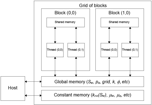
The kernel functions are executed in parallel by threads. These threads are defined by global indexes that belong to a grid of blocks. The grid and block sizes are defined by the user. The grid can be defined for 1, 2 or 3 dimensions. Each block has a finite number of threads, usually up to 1024 thread count. The maximum grid size is given by the manufacturing specifications of each graphics card. All this features of modern GPUs can be consulted elsewhere in NVIDIA CUDA web site. Taking all this into account, it is only possible to efficiently parallelize numerical codes that do not exceed the number of threads that can be executed in the grid of blocks. On the other hand, it is easy to parallelize functions that execute the same operations over the entries of arrays, since only the threads indexes have to be defined and this definition replaces each loop. As an example of this method, Figures 4 and 5 show an extract of the codes for calculating the Jacobian block corresponding to the residual R o and its derivatives (∂R o /∂p o ), in CPU and GPU respectively.
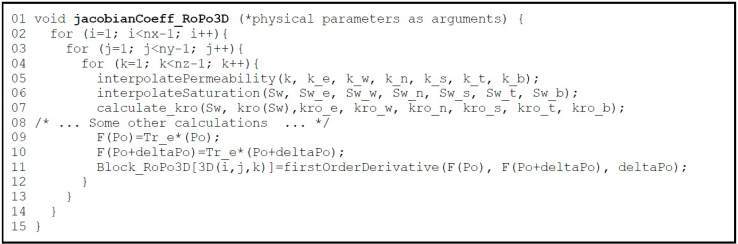

In the function jacobianCoeff_RoPo3D() all the coefficients of Jacobian block ∂R o /∂p o were calculated. The code is standard and is based in tridimensional arrays which contain some variables related to the Cartesian mesh for the numerical simulation. Therefore, three nested cycles occur, one cycle for each axis. In the most internal cycle, several functions are executed to carry out several numerical methods, among them: interpolations for initial relative permeability and saturations from centers of volumes to its faces (lines 5 and 6), calculation of relative permeability using data from tables (line 7), calculations of coefficients of the residual and its derivatives (lines 9 and 10), and the assembling of the corresponding block (line 11).
In the same way as in the Figure 4, in Figure 5 an extract of code of the kernel function is shown that implements the calculation of the Jacobian block ∂R o /∂p o . The kernel function jacobianCoeff_RoPo3D() is executed in the GPU. The first thing to do is to determine the thread index, see lines 2-4. Using this index it is possible that each thread of the block in the grid, execute the operations defined in lines 5-12 concurrently. Line 5 is required to assure that the index is inside the limits of the arrays. Lines 6 to 12 consist of kernel functions, similar to the functions defined in CPU, see Figure 4, but using the index to perform each one of the numerical methods needed to calculate the corresponding block of the Jacobian matrix. These kernels are device functions that can only be executed by another kernel and are able to use the GPU memory (Sanders, 2010; NVIDIA, 2012). Two kind of memories were used: global memory to store the primary variables (S w and p o ), the properties of the porous media (k, φ, etc) and some other important arrays of the simulation; constant memory is used to store constant values, i.e, the viscosities, conversion factors and some tables of properties (relative permeability). Figure 6 shows schematically how the variables are stored within the GPU memory.
Finally, once the Jacobian components has been built, the linear system of equations is constructed in CRS format. This extra step is needed in order to use the algorithms of the EIGEN and CUSP libraries. Both libraries require a matrix in the CRS format and a right hand side (rhs) vector. The result is stored in another vector that contains the solution of the linear system.
Numerical results
As a way to validate the numerical code, in this section numerical results obtained for three different cases are presented. Also numerical performance experiments were carried out to test computationally the parallel numerical code that is compared versus serial code.
Buckley Leverett
The Buckley-Leverett model describes the displacement of oil by water in an horizontal domain. This mathematical model is widely used in the validation of two phase fluid flow simulators, because it has an analytic solution for the water saturation profile. The hypothesis of the Buckley-Leverett model are:
The displacement occurs at a one-dimensional medium.
The porous media is isotropic.
No effects of capillary pressure nor gravity forces are considered.
There are no sources nor sinks.
Water gets injected to a constant flow through the left boundary of the domain. Oil is produced on the right boundary at a constant pressure.
The parameters to carry out the simulation are shown in Table 1. Relative permeabilities k ra (S w ) can be obtained from Chen et al. (2006).
Table 1 Parameters to solve the Buckley-Leverett problem.
| Property | Value |
|---|---|
| Length of domain (L x ) | 1,000 (ft) |
| Absolute permeability (k) | 100.0 (mD) |
| Porosity (ϕ) | 0.20 |
| Water viscosity (μ w ) | 0.42 (cP) |
| Oil viscosity (μ o ) | 15.5 (cP) |
| Residual water saturation (S wr ) | 0.40 |
| Residual oil saturation (S or ) | 0.18 |
| Injection velocity (v inj ) | 2.0E-06 (ft/s) |
| Production pressure (p out ) | 1,000 (psi) |
In this paper a comparison of the analytical solution versus the solution obtained numerically is presented. The numerical parameters were selected as follows: to evaluate the derivatives within the Jacobian blocks increments of ΔSw=1x10 -05 for water saturation and Δpo=0.1 for the oil pressure were used. Stop criterion for leaving the Newton-Rapshon loop was selected to: |δS w | <1x10-05 and a fixed time step of 1 day was chosen. The number of discrete volumes selected to study its effect in the solution were: 100, 500, 1,000, 5,000 and 10,000. The total time simulation was of 120 days and results are saved every 30 days. Table 2 shows a comparison between analytical and numerical solutions at some selected positions. As shown in this table as the number of volumes increases the relative error and the root mean square deviation (RMSD) respect to the analytical solution decreases.
Table 2 Numerical results obtained for the Buckley-Leverett problem.
| Number of discrete volumes | Position x (ft) | Simulation time (days) | Sw Numerical | Sw Analytical domain | Error % | RMSD At the whole |
|---|---|---|---|---|---|---|
| 100 | 145 | 30 | 0.4721 | 0.4 | 18.033 | 0.01510 |
| 275 | 60 | 0.4792 | 0.4 | 19.809 | 0.01590 | |
| 405 | 90 | 0.4801 | 0.4 | 20.037 | 0.01598 | |
| 535 | 120 | 0.4786 | 0.4 | 19.666 | 0.01875 | |
| 500 | 145 | 30 | 0.42238 | 0.4 | 5.5942 | 0.01127 |
| 275 | 60 | 0.42049 | 0.4 | 5.1216 | 0.01095 | |
| 405 | 90 | 0.40972 | 0.4 | 2.4295 | 0.01104 | |
| 535 | 120 | 0.40849 | 0.4 | 2.1213 | 0.001093 | |
| 1,000 | 145 | 30 | 0.40784 | 0.4 | 1.9593 | 0.00987 |
| 275 | 60 | 0.40399 | 0.4 | 0.99737 | 0.01027 | |
| 405 | 90 | 0.40080 | 0.4 | 0.19905 | 0.00981 | |
| 535 | 120 | 0.40056 | 0.4 | 0.13941 | 0.00962 | |
| 5,000 | 145 | 30 | 0.40028 | 0.4 | 0.07096 | 0.00944 |
| 275 | 60 | 0.39998 | 0.4 | 0.00525 | 0.00942 | |
| 405 | 90 | 0.39999 | 0.4 | 0.00170 | 0.00897 | |
| 535 | 120 | 0.40001 | 0.4 | 0.00150 | 0.00839 | |
| 10,000 | 145 | 30 | 0.400130 | 0.4 | 0.03159 | 0.00916 |
| 275 | 60 | 0.400020 | 0.4 | 0.00568 | 0.00917 | |
| 405 | 90 | 0.400001 | 0.4 | 0.00093 | 0.00881 | |
| 535 | 120 | 0.400001 | 0.4 | 0.00091 | 0.00827 |
Figure 7 shows the water saturation and pressure profiles obtained for 120 days of total simulation by using 10,000 discrete volumes. Results of the water saturation profile are congruent with the analytical solution (dashed line). This result indicates that the problem has been solved correctly.

Five Spot
The model known as “Five Spot” describes the displacement of oil by water in an isotropic domain, in which a producer well and an injector well are placed in the opposite corners of the domain (See Figure 8). In the Five Spot conceptual model the follow assumptions are considered:
The displacement occurs at a bidimensional domain.
The porous media is isotropic.
The effects of capillary pressure are considered.
There are one source (injector well) and one sink (producer well).
Gravity forces are neglected.

The parameters to carry out the simulation are shown in Table 3. Relative permeabilities k ra (S w ) and capillary pressure p cow can be obtained from Chen et al. (2006).
Table 3 Parameters to solve the Five Spot problem (Chen et al. 2006).
| Property | Value |
|---|---|
| Size of domain (L s ×L y ) | 1,000 × 1,000 (ft) |
| Absolute permeability (k) | 100.0 (mD) |
| Porosity (ϕ) | 0.20 |
| Water viscosity (μ w ) | 0.096 (cP) |
| Oil viscosity (μ o ) | 1.14 (cP) |
| Residual water saturation (S wr ) | 0.22 |
| Residual oil saturation (S or ) | 0.20 |
| Injection pressure |
3,700 (psi) |
| Production pressure |
2,500 (psi) |
For this problem the total time simulation was selected to 8,000 days and the results are reported every 500 days. Numerical parameters are the same to those in the Buckley-Leverett problem. Because there is no analytical solution for this problem, it is validated with the results reported by Chen et al. (2006). Figure 9 a) shows the production of water and oil in reservoir barrels per day (RB/day) throughout the simulation time. In this figure it can be seen that the results reported by Chen et al. (2006) and those obtained in this work have a similar qualitatively behavior. The difference between curves may be due to the numerical techniques used, since Chen et al. (2006) used an adaptive time step with an IMPES scheme. The RMSD obtained for the production curves are 43.88 and 137.94 for oil and water production, respectively. In Figure 9 b) fractional flow (F w ) curves are compared. It can be appreciated that the water cut happens after 1,000 days of simulation, which is almost the same result reported by Chen et al. (2006).
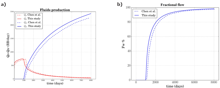
Figure 9 Results obtained using 10 × 10 discrete volumes: a) water and oil productions Qw-Qo in reservoir barrels per day (RB/day); b) fractional flow FW (%).
To verify the solution shape two more simulations were carried out, one considering 30x30 mesh size of and another using 90x90 volumes. Values obtained for RMSD using 30x30 volumes were 41.97 and 135.44; while by using 90x90 volumes were 41.02 and 134.82, for oil and water production respectively.
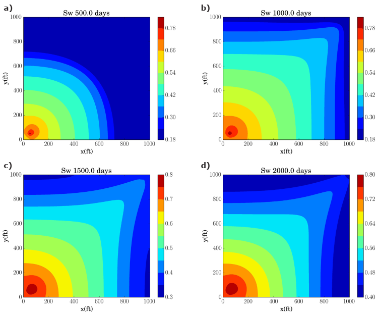
Figure 10 shows the water saturation profiles at different simulation times in the whole numerical domain. This figure is presented in order to clarify how the waterfront sweeps the oil from the porous medium.
The seventh SPE project
The seventh SPE project is a benchmark that describes the water injection and oil production using horizontal wells, this problem was adapted by Nghiem et al. (1991) and Chen et al. (2006) for two-phase fluid flow. In the ´resent case capillary pressure and gravity forces were considered. Therefore equations (10) and (14) are used without any modification.
To solve this problem the SPE proposes a mesh of 10x10x7 (Figure 11). This mesh is refined to the y axis center, in order to place the injection and production wells. The length of the blocks in the x axis are uniform and equal to 300 ft (δx = 300 ft). For the length of the blocks in the y axis, the distribution is as follows: δy 1 = δy 9 = 620 ft, δy 2 = δy 8 = 400 ft, δy 3 = δy 7 = 200 ft, δy 4 = δy 6 = 100 ft and δy 5 = 60 ft. For the z axis δz k = 20 ft for k 1, 2, 3, 4, δz 5 = 30 ft and δz k = 50 ft were used. Injection well is placed in the layer δz 6, at the center of the axis y and it crosses all the blocks in the x axis. Production well is placed in the layer δz 1, at the center of the axis y and it crosses only the blocks δx 6, 7, 8 in the x axis. Parameters to execute the simulation are shown in Table 4. Relative permeabilities k ra (S w ), capillary pressure p cow (S w ), and initial conditions can be obtained from Nghiem et al. (1991).
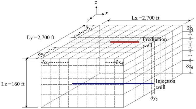
Table 4 Parameters to solve the Seventh SPE project (Nghiem et al. 1991):
| Property | Value |
|---|---|
| Size of domain (L x × L y × L z ) | 2,700 × 2, 700 × 160 (ft) |
| Absolute permeability (k x , k y , k z ) | (300.0, 300.0, 30.0) )mD) |
| Porosity (ϕ) | 0.20 |
| Water viscosity (μ w ) | 0.96 (cP) |
| Oil viscosity (μ o ) | 0.954 (cP) |
| Residual water saturation (S wt ) | 0.22 |
| Residual oil saturation (S or ) | 0.0 |
| Injection pressure |
3,651.4 (psi) |
| Production pressure |
3,513.6 (psi) |
For this problem the total simulation time was selected to be 1,500 days and results are reported every 100 days. Results are validated by comparing production curves reported by Chen et al. (2006). Figure 12 a) shows the oil production in stock tank barrels per day (STB/day) during the entire simulation time. It can be noted that the results are qualitatively similar to those reported by Chen et al. (2006), although the curve reported by them declines slightly faster. The accumulated oil production curves are also compared, these results are shown in Figure 12 b).
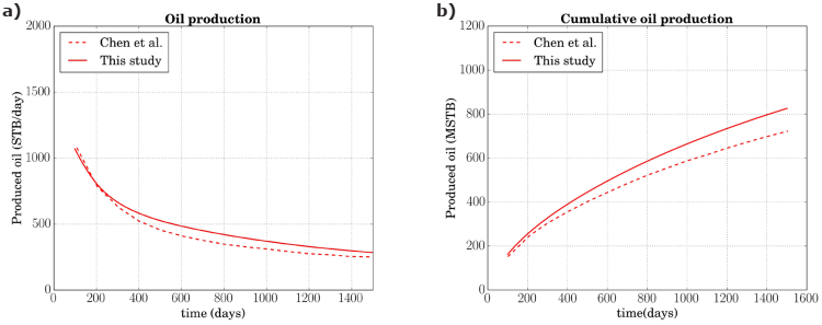
Figure 12 Results obtained using 10×10×7 discrete volumes : a) Oil production (STB/day); b) Cumulative oil production (MSTB).
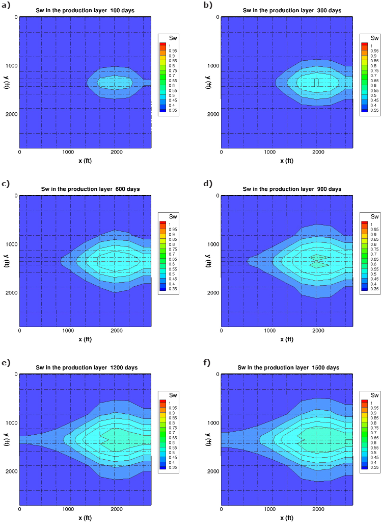
The small difference observed in Figures 12, may be due to implementations of the numerical method and conversion factor used for the STB; in the present work the STB conversion factor from Nghiem et al. (1991) was used. It should be noted that this problem was solved only with the grid size proposed by Nghiem et al. (1991), as it is indicated by this benchmark. The RMSD obtained in this problem is 55.77 for the oil production values and 68.08 for cumulative oil production. In order to know the behavior of the fluids flow in the layer where the production well is placed. Figure 13 shows the saturation profiles S w in this layer for six selected simulation times by using the grid size proposed by Nghiem et al. (1991). For the saturation profiles belonging to 100 and 300 simulation days, it is noted that the water has begun to sweep the oil present in the layer forming a “water feather”. For the 1,200 and 1,500 profiles the water feather has spread out to more than a half the domain. This means that about 40% of the oil present in the layer has already been produced.
Numerical performance experiments
In order to analyze the performance of the numerical code, the five spot water injection problem was selected. Numerical parameters selected were: ΔSw=1x10-05 for water saturation and Δpo=1x10-03 for oil pressure. Stop criterion for leaving the Newton-Rapshon loop was selected to: |δS w | <1x10-03 and a fixed time step of 0.01 day was chosen; results are saved every 1.0 day. 10 days were selected for the total simulation time.
Numerical results presented in this section were obtained by executing our numerical code in a workstation with a single processor Intel (R) i7 (R) CPU 3820 3.60 GHz, 16 Gigabytes of RAM and an NVIDIA Tesla C2075 (R) GPU with 448 cuda-cores and 6 Gigabytes of dedicated memory.
Table 5 shows the average run-time for each Newton-Raphson step. The Jacobian run-time increases considerably when the number of volumes is bigger. As an example, 0.796 s were spended when volumes were 550x550 in CPU, while only 0.0379 s were used on the GPU that means 21x of speed up. This result is a considerable save of computation time taking into account that this procedure has to be repeated every Newton iteration.
Table 5 Average run-time obtained to compute Jacobian.
| Number of volumes | CPU run-time (s) | GPU run-time (s) | Speed up (x) |
|---|---|---|---|
| 30×30 | 0.00284 | 0.00084 | 3.38x |
| 90×90 | 0.02340 | 0.00164 | 14.26x |
| 150×150 | 0.07141 | 0.00311 | 22.96x |
| 250×250 | 0.15049 | 0.00754 | 19.95x |
| 550×550 | 0.79686 | 0.037937 | 21.00x |
Most authors indicate about 75% computation time is consumed in the solution of the system of linear equations. For solving the linear equations system, BICGSTAB solver without a preconditioner was used. This solver is already included in EIGEN and CUSP libraries (Jacob and Guennebaud, 2016; Maia and Dalton, 2016). Run times are shown in Table 6. Results indicate that CPU is faster than GPU when linear system is small (45,000 unknowns). When the linear system increases from 45,000 to 125,000 unknowns the computing time using the GPU is less than CPU. For a system with 605,000 unknowns, the maximum speed up is achieved (2.207x).
Table 6 Average run-time obtained to solve the linear equations system.
| Number of volumes | Unknowns number | CPU run-time (s) | GPU run-time (s) | Speed up (x) |
|---|---|---|---|---|
| 30×30 | 1,800 | 0.007599 | 0.24234 | 0.035x |
| 90×90 | 16,200 | 0.19308 | 0.85252 | 0.226x |
| 150×150 | 45,000 | 0.98792 | 1.0727 | 0.9209x |
| 250×250 | 125,000 | 4.3418 | 2.7515 | 1.570x |
| 550×550 | 605,000 | 29.408 | 13.32 | 2.207x |
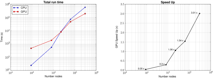
In a numerical code developed with GPU without graphics in real time, numerical results always have to be transfered from GPU to CPU for later processing. This process is computationally expensive because it has to be carried out each time step or when the user requires it. The time measured for this operation was from 1.69x10-05 to 0.101 seconds, for the 30x30 and 550x550 number of volumes, respectively. For this reason real speed up must be quantified when the whole numerical code has finished. Figure 14 shows run time and speed up for executing the whole code. In this figure can be noted GPU is slower than CPU when the problem is executed with few volumes. In the other hand, GPU speed up increases if the number of nodes for executing the problem increases. For executing the numerical code with 302,500 blocks (550x550 number of volumes) 3.0x of speed up is achieved, that is, the total run time for the CPU was 6.8 days whereas for the GPU it was only 2.26 days. It is worth mentioning that in this case the information transfer GPU-CPU does not have a considerable effect, since it was executed only 10 times. It should be kept in mind that this is a benchmark problem, therefore it is not necessary to use a bigger grid size to solve it adequately.
Conclusions
Sequential and parallel implementations of a fully implicit simulator for waterflooding process have been presented. Both implementations were validated with three different benchmarks and similar results were obtained in comparison with other authors and in comparison with analytical solutions. The strategy of parallelization allows to reduce the calculation time of the Jacobian matrix, resulting from the Newton-Raphson method, using the architecture of the GPUs. Numerical results indicate that the GPU implementation reach until 22.9 times faster than the CPU counterpart for the finest mesh. On the other hand, the solution of the final linear system was also carried out in the GPU. A speed up of this step of 2.2 for the finest mesh was ontained. In total, taking into account the construction of the Jacobian matrix, the solution of the linear system and the exchange of information between CPU and GPU, gave a total speed up to 3. As expected, this speed up can be improved as the number of unknowns is incremented, however, the limited number of threads and memory of GPUs is a first obstacle to go forward. Even though the libraries used for solving the linear systems are optimized, they need to be improved with special preconditioners in order to obtain better results in terms of CPU and GPU time, and pair the 22x of speed up that was achieved in the present best calculation of Jacobian matrix. On the other hand, the GPU used in this work is not the newest one in the market, in such a way that a limitation occurs by the number of CUDA cores (448) and the memory (6GB) of the hardware; however, as can be seen, as the size of the problem increase, the speed up improves, therefore if, for example a GPU Tesla K40m (2880 CUDA cores and 12 GB in memory) is used better results can be expected. Finally, the present strategy can be used for several number of GPUs along with domain decomposition methods; this allows to increase even more the size of the problem (to several millions of unknowns) and as a consequence the speed up will be improved. Of course, this requires better solvers for the linear systems, for example geometric or algebraic multigrid methods.

